Struphy 3.1
Structure-Preserving
Hybrid Code

Plasma Models in Python

Stefan Possanner, group for Kinetic-Fluid Hybrid Models

NMPP retreat 2026 - Ammersee

Struphy is …

… an open-source Python package for solving partial differential equations (PDEs), primarily designed for plasma physics — though not limited to it.

💯% Python — Write models in clean, readable Python.

💥 Pyccel-powered kernels — High-performance Fortran code generated via Pyccel.

💻 Simple API — Run complex plasma simulations with minimal boilerplate.

🌐 Open-source & community-driven — Built for collaboration and accessibility.

Numerical methods

Particle-in-cell (PIC) method for kinetic models:

\[ f(t, x, v) = \sum_k w_k\, \delta(x - x_k(t))\, \delta(v - v_k(t)) \]

Finite element exterior calculus (FEEC) for fluid/field variables (via Psydac):

\[ \mathbf E(t, x) = \sum_i e_i(t)\, \mathbf \Lambda^1_i(x)\,, \qquad \mathbf B(t, x) = \sum_i b_i(t)\, \mathbf \Lambda^2_i(x) \]

Smoothed Particle Hydrodynamics (SPH) for fluid models:

\[ n(t, x) = \sum_k w_k\, W(x - x_k(t))\,,\qquad \mathbf u(t, x) = \sum_k \frac{w_k}{n(t, x_k(t))}\, \mathbf v_k(t)\, W(x - x_k(t)) \]

Struphy provides MPI/OpenMP data structures for these methods (GPU via cuda-python in the second half of 2026 - ACH project 6 months).

Under consideration: Hermite polynomials for velocity discretization (C. Negulescu)

Purpose of Struphy

Provide a common Python API for researchers working on plasma physics PDEs

(such a thing exists for quantum physics, check out QuTiP).

Care about maintainable code, avoid “technical debt” in research software

Instead of losing research code, provide a framework for its preservation and reuse.

Enable computational plasma research for a wider audience, including students and researchers that are not experts in programming.

Current team

Amin Raissi (PhD student with Omar Maj): SPH discretization of viscous Euler equations
Lorenzo Mazzi (Master student with Omar Maj): high frequency decomposition in Euler-Maxwell equations
Emile Grivet (4 month intership from Paris-Saclay): Benchmarking ITG turbulence with drift-kinetic equations in Struphy
David Székedi (internship from TU delft, remote): saddle point problem for quasi-neutral two-fluid equations
Max Lindqvist (ACH): Maintainer

Getting the code

Installation Options

Install on bare metal (Linux/macOS)
1. From PyPI (recommended)
2. From source (for development)
Use Docker (cross-platform)
Run tutorials on Binder (cloud-based)

🌐 Repo: github.com/struphy-hub/struphy

🌐 Docs: struphy-hub.github.io/struphy

🌐 Tutorials: github.com/struphy-hub/struphy-tutorials

Install on bare metal (Linux/macOS)

Use a virtual environment:

python -m venv struphy-env
source struphy-env/bin/activate

From PyPI (with physics packages and MPI support):

pip install -U struphy[phys,mpi]

From source (for development):

git clone https://github.com/struphy-hub/struphy.git
cd struphy
pip install -e .[phys,dev]

Compile kernels (Fortran code generated via Pyccel):

struphy compile

Use Docker (cross-platform)

Pull the latest image from Docker Hub and run it:

docker pull spossann/struphy:main
docker run -it --rm spossann/struphy:main

List the existing environments and activate one:

ls struphy_*
source struphy_fortran_/env_fortran_/bin/activate
struphy -v

Check the compilation:

struphy compile --status

Run tutorials on Binder (cloud-based)

🌐 Tutorials: github.com/struphy-hub/struphy-tutorials

Run examples

Visit the repo for example parameter files:

🌐 Repo: github.com/struphy-hub/struphy-parameter-files

Easy to launch and post-process examples:

cd VlasovAmpereOneSpecies
cd two_stream
python params_two_stream.py
python pproc_two_stream.py

Getting started

Check version in CLI

struphy -v

Struphy 3.1.0
Copyright 2019-2026 (c) Struphy dev team | Max Planck Institute for Plasma Physics
MIT license

Get more info in CLI:

struphy --help

usage: struphy [-h] [-v] [-s] [--fluid] [--kinetic] [--hybrid] COMMAND ...

Struphy: STRUcture-Preserving HYbrid code for plasma physics.

options:
  -h, --help        show this help message and exit
  -v, --version     show program's version number and exit
  -s, --short-help  display short help
  --fluid           display available fluid models
  --kinetic         display available kinetic models
  --hybrid          display available hybrid models

available commands:
  compile           compile computational kernels (including psydac)
  params            create default parameter file for a model, or show model's options
  profile           profile finished runs
  test              run tests
  format            format source files
  lint              lint and analyze source files

Type "struphy COMMAND --help" for more information on a command.

For more help on how to use Struphy, see https://struphy-hub.github.io/struphy/

Import model

from struphy.models import Maxwell

Maxwell.info()

Maxwell's equations in vacuum for electromagnetic field evolution.

To see detailed information on the model, run the following methods:

Maxwell.pde()
Maxwell.normalization()
Maxwell.scalar_quantities()
Maxwell.discretization()
Maxwell.long_description()
Maxwell.examples()
Maxwell.use_cases()
Maxwell.cannot_be_used_for()

Maxwell.pde()

PDEs solved by model:

Ampère's law (no current):

∂𝐄∂t - ∇ × 𝐁 = 0

Faraday's law:

∂𝐁∂t + ∇ × 𝐄 = 0

Maxwell.normalization()

Normalization:

Velocity and fields are normalized as:

v̂ = c , Ê = c B̂

where c is the speed of light.

Maxwell.scalar_quantities()

The following scalars are tracked during simulation:

Electric energy: E_E = ¹⁄₂ ∫ |𝐄|² dV
Magnetic energy: E_B = ¹⁄₂ ∫ |𝐁|² dV
Total energy: Eₜₒₜₐₗ = E_E + E_B

Maxwell.discretization()

Discretization (Propagators called in sequence):

1. propagators_fields.Maxwell:

FEEC discretization of the following equations: find 𝐄 ∈ H(curl) and 𝐁 ∈ H(div) such that

∫_Ω ∂𝐄∂t · 𝐅 d 𝐱 - ∫_Ω 𝐁 · ∇ × 𝐅 d 𝐱	=0 , ∀ 𝐅 ∈ H(curl)
∂𝐁∂t + ∇×𝐄	=0 .

Time discretization:

implicit: Crank-Nicolson (implicit mid-point)
explicit: explicit RK methods from ButcherTableau

System size reduction via struphy.linear_algebra.schur_solver.SchurSolver.

Run a Simulation

from struphy import Simulation

model = Maxwell()
sim = Simulation(model=model)

Run the simulation:

sim.run()


Starting simulation run for model Maxwell ...
Struphy run finished.

Post-process the simulation:

sim.pproc()

  0%|          | 0/2 [00:00<?, ?it/s]100%|██████████| 2/2 [00:00<00:00, 252.55it/s]
  0%|          | 0/4 [00:00<?, ?it/s]100%|██████████| 4/4 [00:00<00:00, 472.88it/s]
  0%|          | 0/4 [00:00<?, ?it/s]100%|██████████| 4/4 [00:00<00:00, 881.39it/s]

Load plotting data

sim.load_plotting_data()

Run more verbosely

from struphy import set_logging_level
import logging

set_logging_level(logging.INFO)

sim = Simulation(model=model)
sim.run()


Starting simulation run for model Maxwell ...

PROPAGATOR OPTIONS:

Options for propagator 'Maxwell':
    algo:               implicit
    solver:             pcg
    precond:            MassMatrixPreconditioner
    solver_params:      SolverParameters(tol=1e-08, maxiter=3000, info=False, verbose=False, recycle=True)
    butcher:            None

INITIAL CONDITIONS:

Variable 'e_field' of species 'EMFields' - no background.

Variable 'e_field' of species 'EMFields' - no perturbation.

Variable 'b_field' of species 'EMFields' - no background.

Variable 'b_field' of species 'EMFields' - no perturbation.

Allocating simulation data ...

WARNING: Class "BasisProjectionOperators" called with degree=(1, 1, 1) (interpolation of piece-wise constants should be avoided).

Allocated SplineFuntion 'e_field' in space 'Hcurl'.

Allocated SplineFuntion 'b_field' in space 'Hdiv'.

Rank 0: executing run() for model Maxwell ...

INITIAL SCALAR QUANTITIES:
electric_energy:                          0.00e+00
magnetic_energy:                          0.00e+00
total_energy:                             0.00e+00


START TIME STEPPING WITH 'LieTrotter' SPLITTING:
time step:                                     1/3
normalized time:               1.00e-02 / 3.00e-02
physical time [s]:             3.34e-11 / 1.00e-10
wall clock time [s]:                        0.2221
last step duration [s]:                     0.0098
electric_energy:                          0.00e+00
magnetic_energy:                          0.00e+00
total_energy:                             0.00e+00

time step:                                     2/3
normalized time:               2.00e-02 / 3.00e-02
physical time [s]:             6.67e-11 / 1.00e-10
wall clock time [s]:                        0.2467
last step duration [s]:                     0.0102
electric_energy:                          0.00e+00
magnetic_energy:                          0.00e+00
total_energy:                             0.00e+00

time step:                                     3/3
normalized time:               3.00e-02 / 3.00e-02
physical time [s]:             1.00e-10 / 1.00e-10
wall clock time [s]:                        0.2637
last step duration [s]:                     0.0092
electric_energy:                          0.00e+00
magnetic_energy:                          0.00e+00
total_energy:                             0.00e+00


Time steps done: 3
wall-clock time of simulation [sec]: 0.27837443351745605

Struphy run finished.

Post-process the simulation:

sim.pproc()


Post-processing path /home/IPP-AD/spossann/git_repos/2026_NMPP_retreat/sim_1

Reading hdf5 data of following species:
em_fields:
  b_field: <HDF5 group "/feec/em_fields/b_field" (3 members)>
  e_field: <HDF5 group "/feec/em_fields/e_field" (3 members)>

Allocated SplineFuntion 'b_field' in space 'Hdiv'.

Allocated SplineFuntion 'e_field' in space 'Hcurl'.

Allocated SplineFuntion 'b_field' in space 'Hdiv'.

Allocated SplineFuntion 'e_field' in space 'Hcurl'.

Allocated SplineFuntion 'b_field' in space 'Hdiv'.

Allocated SplineFuntion 'e_field' in space 'Hcurl'.

Allocated SplineFuntion 'b_field' in space 'Hdiv'.

Allocated SplineFuntion 'e_field' in space 'Hcurl'.

  0%|          | 0/2 [00:00<?, ?it/s]100%|██████████| 2/2 [00:00<00:00, 257.67it/s]
Creation of Struphy Fields done.

Evaluating fields ...
  0%|          | 0/4 [00:00<?, ?it/s]100%|██████████| 4/4 [00:00<00:00, 419.24it/s]

Creating vtk in /home/IPP-AD/spossann/git_repos/2026_NMPP_retreat/sim_1/post_processing/fields_data ...
  0%|          | 0/4 [00:00<?, ?it/s]100%|██████████| 4/4 [00:00<00:00, 610.30it/s]

No kinetic data found in hdf5 file, skipping post-processing of kinetic data.

Load plotting data

sim.load_plotting_data()


Loading post-processed plotting data:
Data path: /home/IPP-AD/spossann/git_repos/2026_NMPP_retreat/sim_1/post_processing

Files in /home/IPP-AD/spossann/git_repos/2026_NMPP_retreat/sim_1/post_processing/fields_data/em_fields: ['e_field_log.bin', 'b_field_log.bin']

The following data has been loaded:

grids:
self.t_grid.shape =(4,)
self.grids_log[0].shape =(25,)
self.grids_log[1].shape =(11,)
self.grids_log[2].shape =(2,)
self.grids_phy[0].shape =(25, 11, 2)
self.grids_phy[1].shape =(25, 11, 2)
self.grids_phy[2].shape =(25, 11, 2)

self.spline_values:
    em_fields
        e_field_log
        b_field_log

self.orbits:

self.f:

self.n_sph:

Poisson tutorial (written by copilot)

Solving 1D Poisson with periodic boundary conditions in Struphy

This tutorial shows how to solve a manufactured 1D Poisson problem with the Poisson model.

We use a periodic domain \(x \in [0, L)\) and choose an analytic solution

\[ \phi_\mathrm{exact}(x) = \cos(kx), \]

so the source for the stabilized Poisson problem

\[ -\phi'' + \varepsilon\phi = \rho \]

\[ \rho(x) = (k^2 + \varepsilon)\cos(kx). \]

Then we run a Struphy Simulation, compare numerical and exact solutions, and compute the max-norm error.

import numpy as np
import matplotlib.pyplot as plt

from struphy import Simulation, DerhamOptions, domains, grids, perturbations
from struphy.initial.base import GenericPerturbation
from struphy.models import Poisson

Poisson.pde()

PDEs solved by model:

Find φ ∈ H¹ such that

-∇ · D₀(𝐱) ∇ φ + n₀(𝐱) φ = ρ(t, 𝐱)

where n₀, ρ(t) : Ω → ℝ are real-valued functions, ρ(t) is

parametrized by time t, and D₀ : Ω → ℝ^{3 × 3} is a positive matrix.

Boundary terms from integration by parts are assumed to vanish.

# Manufactured periodic test case in 1D (aligned with verification test pattern)
Lx = 2.0 * np.pi
mode = 2
k = mode * 2.0 * np.pi / Lx

# Tiny stabilization makes the periodic problem uniquely solvable
stab_eps = 1e-8

# Build the source through the model variable as in test_verif_Poisson.py
model = Poisson()

options = model.propagators.poisson.Options(
    rho=model.em_fields.source,
    stab_eps=stab_eps,
    )
model.propagators.poisson.options = options

source_amp = k**2 + stab_eps
model.em_fields.source.add_perturbation(
    perturbations.ModesCos(ls=(mode,), amps=(source_amp,))
    )

phi_exact = lambda e1, e2, e3: np.cos(k * e1)

Poisson.Options controls the elliptic solve. In this example we only set:

rho: the manufactured source term.
stab_eps: a tiny stabilization to remove the constant null-space in the periodic case.

All other option fields are left at their defaults (solver choice, preconditioner, tolerances, etc.).

# 1D periodic setup: periodic bcs are the default (None in each direction)
domain = domains.Cuboid(l1=0.0, r1=Lx)
grid = grids.TensorProductGrid(num_elements=(64, 1, 1))
derham_opts = DerhamOptions()

sim = Simulation(
    model=model,
    domain=domain,
    grid=grid,
    derham_opts=derham_opts,
    )

# For a stationary Poisson solve, one time step is enough
set_logging_level(logging.WARNING)
sim.run(one_time_step=True)
sim.pproc()
set_logging_level(logging.INFO)
sim.load_plotting_data()


Starting simulation run for model Poisson ...
Struphy run finished.
  0%|          | 0/2 [00:00<?, ?it/s]100%|██████████| 2/2 [00:00<00:00, 753.56it/s]
  0%|          | 0/2 [00:00<?, ?it/s]100%|██████████| 2/2 [00:00<00:00, 1437.14it/s]
  0%|          | 0/2 [00:00<?, ?it/s]100%|██████████| 2/2 [00:00<00:00, 1722.86it/s]

Loading post-processed plotting data:
Data path: /home/IPP-AD/spossann/git_repos/2026_NMPP_retreat/sim_1/post_processing

Files in /home/IPP-AD/spossann/git_repos/2026_NMPP_retreat/sim_1/post_processing/fields_data/em_fields: ['phi_log.bin', 'source_log.bin']

The following data has been loaded:

grids:
self.t_grid.shape =(2,)
self.grids_log[0].shape =(65,)
self.grids_log[1].shape =(2,)
self.grids_log[2].shape =(2,)
self.grids_phy[0].shape =(65, 2, 2)
self.grids_phy[1].shape =(65, 2, 2)
self.grids_phy[2].shape =(65, 2, 2)

self.spline_values:
    em_fields
        phi_log
        source_log

self.orbits:

self.f:

self.n_sph:

# Extract 1D line data and compare to analytic solution
x = sim.grids_phy[0][:, 0, 0]

t_last = max(sim.spline_values.em_fields.phi_log.data.keys())
phi_num = sim.spline_values.em_fields.phi_log.data[t_last][0][:, 0, 0]
phi_ref = phi_exact(x, 0.0, 0.0)

err = phi_num - phi_ref
err_max = np.max(np.abs(err))

max-norm error ||phi_h - phi_exact||_inf = 3.207e-03
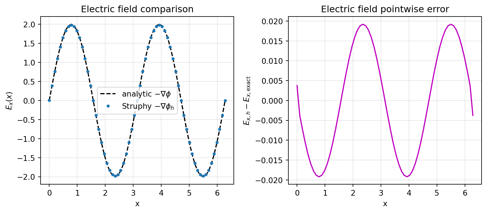
max-norm error ||E_h - E_exact||_inf = 1.920e-02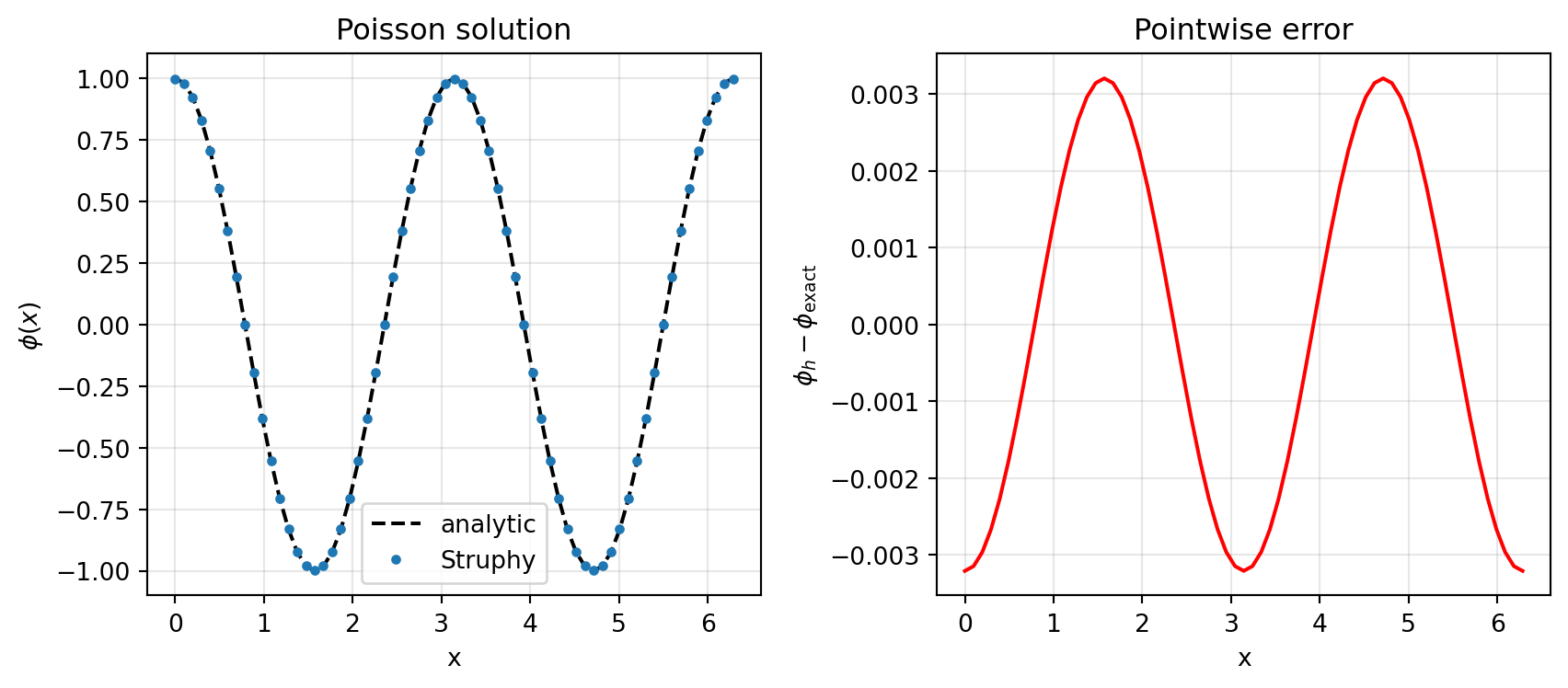

Poisson tutorial (contd.)

2D Manufactured Test on a Rectangle

We now solve a 2D manufactured Poisson problem on a rectangle with different side lengths:

\[ (x,y) \in [0,L_x] \times [0,L_y], \qquad L_x \neq L_y. \]

Choose

\[ \phi_\mathrm{exact}(x,y) = \sin\left(\frac{2\pi x}{L_x}\right)\sin\left(\frac{2\pi y}{L_y}\right), \]

which satisfies homogeneous Dirichlet conditions on all rectangle boundaries. For

\[ -\Delta\phi + \varepsilon\phi = \rho, \]

the manufactured source is

\[ \rho(x,y) = \left[\left(\frac{2\pi}{L_x}\right)^2 + \left(\frac{2\pi}{L_y}\right)^2 + \varepsilon\right] \phi_\mathrm{exact}(x,y). \]

To stay consistent with Struphy’s source handling, we build this source through a model perturbation.

# 2D manufactured Poisson setup and solve
Lx2 = 2.0
Ly2 = 1.0
eps2 = 1e-8

kx2 = 2.0 * np.pi / Lx2
ky2 = 2.0 * np.pi / Ly2

phi2_exact = lambda e1, e2, e3: np.sin(kx2 * e1) * np.sin(ky2 * e2)

model2 = Poisson()
model2.propagators.poisson.options = model2.propagators.poisson.Options(
    rho=model2.em_fields.source,
    stab_eps=eps2,
    )

source_amp2 = kx2**2 + ky2**2 + eps2
model2.em_fields.source.add_perturbation(
    perturbations.ModesSinSin(ls=(1,), ms=(1,), amps=(source_amp2,))
    )

domain2 = domains.Cuboid(l1=0.0, r1=Lx2, l2=0.0, r2=Ly2)
grid2 = grids.TensorProductGrid(num_elements=(48, 32, 1))
derham_opts2 = DerhamOptions(
    degree=(3, 3, 1),
    bcs=(("dirichlet", "dirichlet"), ("dirichlet", "dirichlet"), None),
    )

sim2 = Simulation(
    model=model2,
    domain=domain2,
    grid=grid2,
    derham_opts=derham_opts2,
    )

set_logging_level(logging.WARNING)
sim2.run(one_time_step=True)
sim2.pproc()
sim2.load_plotting_data()


Starting simulation run for model Poisson ...
Struphy run finished.
  0%|          | 0/2 [00:00<?, ?it/s]100%|██████████| 2/2 [00:00<00:00, 534.78it/s]
  0%|          | 0/2 [00:00<?, ?it/s]100%|██████████| 2/2 [00:00<00:00, 305.13it/s]
  0%|          | 0/2 [00:00<?, ?it/s]100%|██████████| 2/2 [00:00<00:00, 206.84it/s]

# 2D diagnostics and plots
t2_last = max(sim2.spline_values.em_fields.phi_log.data.keys())
X = sim2.grids_phy[0][:, :, 0]
Y = sim2.grids_phy[1][:, :, 0]

phi2_num = sim2.spline_values.em_fields.phi_log.data[t2_last][0][:, :, 0]
phi2_ref = phi2_exact(X, Y, 0.0)
err2 = phi2_num - phi2_ref
err2_max = np.max(np.abs(err2))

2D max-norm error ||phi_h - phi_exact||_inf = 1.589e-07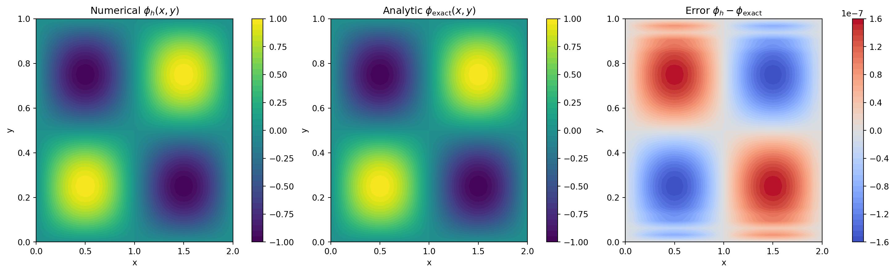

Poisson tutorial (contd.)

2D Manufactured Test on a Thin Annulus (HollowCylinder)

As a second 2D geometry test, we solve Poisson on a disc-shaped domain with a small hole, i.e. a thin annulus.

We use the physical manufactured solution

\[ \phi_\mathrm{exact}(r,\theta)=\sin\!\left(\pi\frac{r-a_1}{a_2-a_1}\right)\sin(m\theta), \]

with \(r=\sqrt{x^2+y^2}\) and \(\theta=\mathrm{atan2}(y,x)\). This vanishes at \(r=a_1\) and \(r=a_2\), so we impose homogeneous Dirichlet conditions in the radial direction.

For

\[ -\Delta\phi + \varepsilon\phi = \rho, \]

the source \(\rho\) is computed analytically in polar coordinates and injected as a physical-space perturbation.

Below, all plots are shown in physical coordinates \((x,y)\) only.

# HollowCylinder manufactured annulus test (physical-space definition)
a1 = 0.8
a2 = 1.0
Lz3 = 1.0
m3 = 3
eps3 = 1e-8
w3 = a2 - a1
alpha3 = np.pi / w3

def phi3_exact(x, y, z):
    r = np.sqrt(x**2 + y**2)
    theta = np.arctan2(y, x)
    s = alpha3 * (r - a1)
    return np.sin(s) * np.sin(m3 * theta)

def rho3_exact(x, y, z):
    r = np.sqrt(x**2 + y**2)
    theta = np.arctan2(y, x)
    s = alpha3 * (r - a1)

    sin_s = np.sin(s)
    cos_s = np.cos(s)
    sin_mt = np.sin(m3 * theta)

    # -Delta(phi) + eps*phi for phi(r,theta)=sin(s)sin(m theta)
    term = (alpha3**2) * sin_s - (alpha3 / r) * cos_s + (m3**2 / r**2) * sin_s + eps3 * sin_s
    return term * sin_mt

model3 = Poisson()
model3.propagators.poisson.options = model3.propagators.poisson.Options(
    rho=model3.em_fields.source,
    stab_eps=eps3,
    )

model3.em_fields.source.add_perturbation(
    GenericPerturbation(rho3_exact, given_in_basis="physical")
    )

domain3 = domains.HollowCylinder(a1=a1, a2=a2, Lz=Lz3)
grid3 = grids.TensorProductGrid(num_elements=(36, 96, 1))
derham_opts3 = DerhamOptions(
    degree=(3, 3, 1),
    bcs=(("dirichlet", "dirichlet"), None, None),
    )

sim3 = Simulation(
    model=model3,
    domain=domain3,
    grid=grid3,
    derham_opts=derham_opts3,
    )

sim3.run(one_time_step=True)
sim3.pproc()
sim3.load_plotting_data()


Starting simulation run for model Poisson ...
Struphy run finished.
  0%|          | 0/2 [00:00<?, ?it/s]100%|██████████| 2/2 [00:00<00:00, 1006.43it/s]
  0%|          | 0/2 [00:00<?, ?it/s]100%|██████████| 2/2 [00:00<00:00, 115.67it/s]
  0%|          | 0/2 [00:00<?, ?it/s]100%|██████████| 2/2 [00:00<00:00, 78.55it/s]

# Annulus diagnostics and plots in physical coordinates only
t3_last = max(sim3.spline_values.em_fields.phi_log.data.keys())
X3 = sim3.grids_phy[0][:, :, 0]
Y3 = sim3.grids_phy[1][:, :, 0]

phi3_num = sim3.spline_values.em_fields.phi_log.data[t3_last][0][:, :, 0]
phi3_ref = phi3_exact(X3, Y3, 0.0)
err3 = phi3_num - phi3_ref
err3_max = np.max(np.abs(err3))

Annulus max-norm error ||phi_h - phi_exact||_inf = 1.101e-05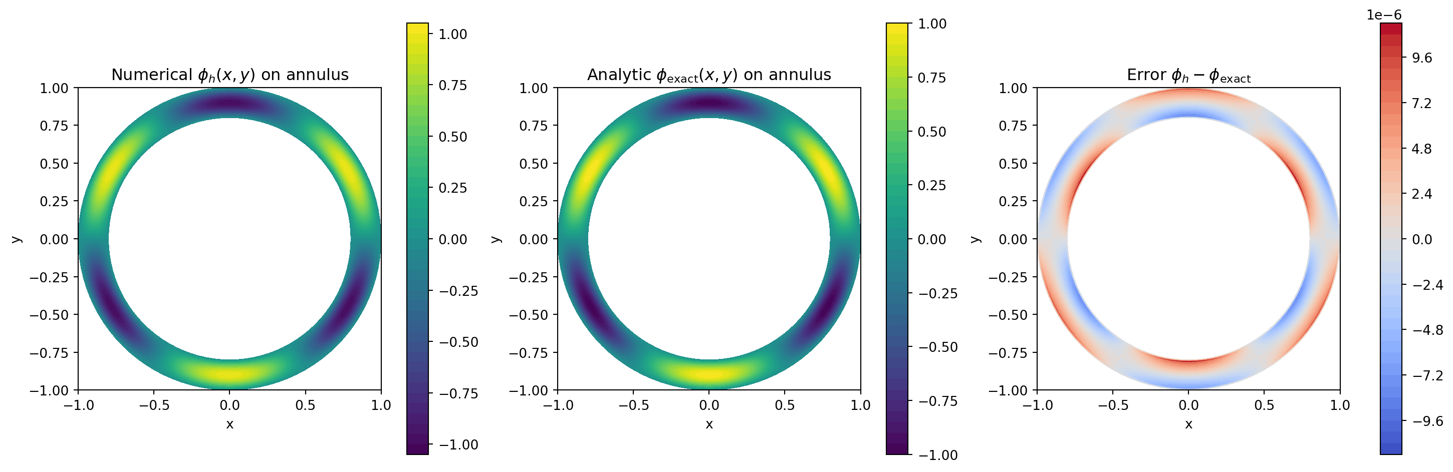

Building models - the Lego system

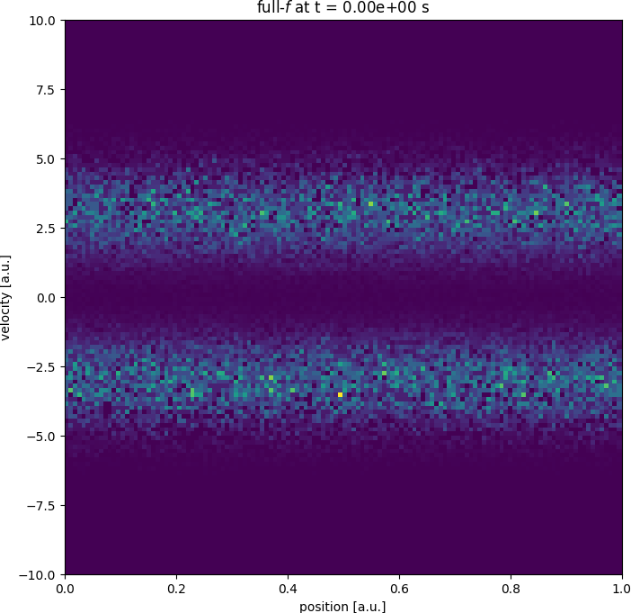
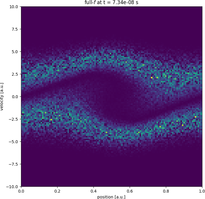
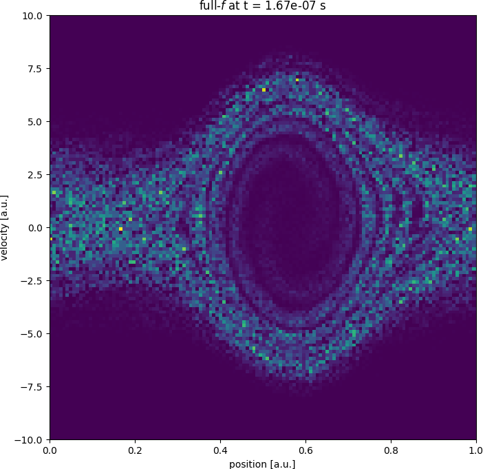
Vlasov

from struphy.models import Vlasov

Vlasov.pde()

PDEs solved by model:

Vlasov equation:

∂f∂t + 𝐯 · ∇ f + ( 𝐯 × 𝐁₀ ) · ∂f∂𝐯 = 0

Vlasov.discretization()

Discretization (Propagators called in sequence):

1. propagators_markers.PushVxB:

For each marker p, solves

d 𝐯ₚ(t)d t = 1ε 𝐯ₚ(t) × (𝐁 + 𝐁_add) ,

where ε = 1/(Ω̂_c t̂) is a constant scaling factor, and for rotation vector 𝐁 and optional, additional fixed rotation vector 𝐁_add, both given as a 2-form:

𝐁 = DF B̂²√g .

Available algorithms:

analytic
implicit.

2. propagators_markers.PushEta:

For each marker p, solves

d 𝐱ₚ(t)d t = 𝐯ₚ ,

for constant 𝐯ₚ in logical space given by 𝐱 = F(η):

d ηₚ(t)d t = DF⁻¹(ηₚ(t)) 𝐯ₚ .

Available algorithms:

Explicit RK from struphy.ode.utils.ButcherTableau

Vlasov-Ampere

from struphy.models import VlasovAmpereOneSpecies

VlasovAmpereOneSpecies.pde()

PDEs solved by model:

Vlasov equation:

∂f∂t + 𝐯 · ∇ f + 1ε ( 𝐄 + 𝐯 × 𝐁₀ ) · ∂f∂𝐯 = 0

Ampère's law:

-∂𝐄∂t = α²ε ∫_ℝ³ 𝐯 f d³ 𝐯

Initial Poisson equation: At t=0, solve weakly for the electric potential φ:

∫_Ω ∇ ψ^→p · ∇ φ d 𝐱	=α²ε ∫_Ω ∫_ℝ³ ψ (f - f₀) d³ 𝐯 d 𝐱 ∀ ψ ∈ H¹
𝐄(t=0)	=-∇ φ(t=0)

VlasovAmpereOneSpecies.discretization()

Discretization (Propagators called in sequence):

Time integration is performed by the following propagators (in sequence):

1. propagators_markers.PushEta:

For each marker p, solves

d 𝐱ₚ(t)d t = 𝐯ₚ ,

for constant 𝐯ₚ in logical space given by 𝐱 = F(η):

d ηₚ(t)d t = DF⁻¹(ηₚ(t)) 𝐯ₚ .

Available algorithms:

Explicit RK from struphy.ode.utils.ButcherTableau

2. propagators_markers.PushVxB:

For each marker p, solves

d 𝐯ₚ(t)d t = 1ε 𝐯ₚ(t) × (𝐁 + 𝐁_add) ,

where ε = 1/(Ω̂_c t̂) is a constant scaling factor, and for rotation vector 𝐁 and optional, additional fixed rotation vector 𝐁_add, both given as a 2-form:

𝐁 = DF B̂²√g .

Available algorithms:

analytic
implicit.

3. propagators_coupling.VlasovAmpere:

PIC-FEEC discretization of the following equations: find 𝐄 ∈ H(curl) and f such that

-∫_Ω ∂𝐄∂t · 𝐅 d 𝐱	=α²ε ∫_Ω ∫_ℝ³ f 𝐯 · 𝐅 d³ 𝐯 d 𝐱 ∀ 𝐅 ∈ H(curl)
∂f∂t + 1ε 𝐄 · ∂f∂𝐯	=0 .

Time discretization: Crank-Nicolson (implicit mid-point).

System size reduction via struphy.linear_algebra.schur_solver.SchurSolver.

Vlasov-Maxwell

from struphy.models import VlasovMaxwellOneSpecies

VlasovMaxwellOneSpecies.pde()

PDEs solved by model:

Vlasov equation:

∂f∂t + 𝐯 · ∇ f + 1ε ( 𝐄 + 𝐯 × ( 𝐁 + 𝐁₀ ) ) · ∂f∂𝐯 = 0

Ampère's law:

-∂𝐄∂t + ∇ × 𝐁 = α²ε ∫_ℝ³ 𝐯 f d³ 𝐯

Faraday's law:

∂𝐁∂t + ∇ × 𝐄 = 0

where Z=-1 and A=1/1836 for electrons.

At initial time the weak Poisson equation is solved once to weakly satisfy Gauss' law,

∫_Ω ∇ ψ^→p · ∇ φ d 𝐱	=α²ε ∫_Ω ∫_ℝ³ ψ (f - f₀) d³ 𝐯 d 𝐱 ∀ ψ ∈ H¹
𝐄(t=0)	=-∇ φ(t=0)

Moreover, it is assumed that

∇ × 𝐁₀ = α²ε ∫_ℝ³ 𝐯 f₀ d³ 𝐯

where 𝐁₀ is the static equilibrium magnetic field.

VlasovMaxwellOneSpecies.discretization()

Discretization (Propagators called in sequence):

1. propagators_fields.Maxwell:

FEEC discretization of the following equations: find 𝐄 ∈ H(curl) and 𝐁 ∈ H(div) such that

∫_Ω ∂𝐄∂t · 𝐅 d 𝐱 - ∫_Ω 𝐁 · ∇ × 𝐅 d 𝐱	=0 , ∀ 𝐅 ∈ H(curl)
∂𝐁∂t + ∇×𝐄	=0 .

Time discretization:

implicit: Crank-Nicolson (implicit mid-point)
explicit: explicit RK methods from ButcherTableau

System size reduction via struphy.linear_algebra.schur_solver.SchurSolver.

2. propagators_markers.PushEta:

For each marker p, solves

d 𝐱ₚ(t)d t = 𝐯ₚ ,

for constant 𝐯ₚ in logical space given by 𝐱 = F(η):

d ηₚ(t)d t = DF⁻¹(ηₚ(t)) 𝐯ₚ .

Available algorithms:

Explicit RK from struphy.ode.utils.ButcherTableau

3. propagators_markers.PushVxB:

For each marker p, solves

d 𝐯ₚ(t)d t = 1ε 𝐯ₚ(t) × (𝐁 + 𝐁_add) ,

where ε = 1/(Ω̂_c t̂) is a constant scaling factor, and for rotation vector 𝐁 and optional, additional fixed rotation vector 𝐁_add, both given as a 2-form:

𝐁 = DF B̂²√g .

Available algorithms:

analytic
implicit.

4. propagators_coupling.VlasovAmpere:

PIC-FEEC discretization of the following equations: find 𝐄 ∈ H(curl) and f such that

-∫_Ω ∂𝐄∂t · 𝐅 d 𝐱	=α²ε ∫_Ω ∫_ℝ³ f 𝐯 · 𝐅 d³ 𝐯 d 𝐱 ∀ 𝐅 ∈ H(curl)
∂f∂t + 1ε 𝐄 · ∂f∂𝐯	=0 .

Time discretization: Crank-Nicolson (implicit mid-point).

System size reduction via struphy.linear_algebra.schur_solver.SchurSolver.

Summary

Takeaways (by copilot)

Struphy is designed to make advanced plasma simulation methods composable, performant, and reusable.

Flexibility by design: particle methods, FEEC-based field discretizations, SPH ideas, multiple geometries, and different model ingredients can live in one common framework.

A Lego system for models: equations, propagators, couplings, grids, domains, and post-processing tools can be combined and recombined instead of reimplemented for every new code.

Performance where it matters: high-level Python interfaces are paired with compiled kernels via Pyccel and parallel data structures built for MPI/OpenMP workflows.

Reusable research software: once a method is implemented in Struphy, it becomes easier to test, extend, benchmark, preserve, and share across projects and generations of users.

Goal: turn specialized plasma codes into a sustainable ecosystem of interoperable building blocks.

Struphy 3.1 Structure-Preserving Hybrid Code

Struphy is …

Numerical methods

Purpose of Struphy

Current team

Getting the code

Installation Options

Install on bare metal (Linux/macOS)

Use Docker (cross-platform)

Run tutorials on Binder (cloud-based)

Run examples

Getting started

Check version in CLI

Import model

Maxwell's equations in vacuum for electromagnetic field evolution.

PDEs solved by model:

Normalization:

The following scalars are tracked during simulation:

Discretization (Propagators called in sequence):

1. propagators_fields.Maxwell:

Run a Simulation

Run more verbosely

Poisson tutorial (written by copilot)

PDEs solved by model:

Poisson tutorial (contd.)

Poisson tutorial (contd.)

Building models - the Lego system

Vlasov

PDEs solved by model:

Discretization (Propagators called in sequence):

1. propagators_markers.PushVxB:

2. propagators_markers.PushEta:

Vlasov-Ampere

PDEs solved by model:

Discretization (Propagators called in sequence):

1. propagators_markers.PushEta:

2. propagators_markers.PushVxB:

3. propagators_coupling.VlasovAmpere:

Vlasov-Maxwell

PDEs solved by model:

Discretization (Propagators called in sequence):

1. propagators_fields.Maxwell:

2. propagators_markers.PushEta:

3. propagators_markers.PushVxB:

4. propagators_coupling.VlasovAmpere:

Summary

Takeaways (by copilot)

Struphy 3.1
Structure-Preserving
Hybrid Code