Meshless
Structure-Preserving
Algorithms

SPEGEO: Structure-Preserving Algorithms and Geometric Numerical Integration school

Stefan Possanner

Max Planck Institute for Plasma Physics, Garching, Germany

June 22-26, 2026 · Strasbourg

Course overview

• Part I: Theory - From Lagrangian to Eulerian coordinates via Euler-Poincaré reduction

  1. Variational principles vs. Newtonian mechanics
  2. Variational principles in fluid mechanics (field theories)
  3. Lagrangian vs. Eulerian descriptions of fluid motion
  4. Euler-Poincaré reduction

• Part II: Discretization - Particle methods for fluid Lagrangians

  5. Functions (0-forms) and volume forms
  6. Discrete Lagrangians
  7. Smoothed-particle hydrodynamics (SPH)

• Part III: Software - Solving meshfree discretizations with Struphy

  8. Struphy: an open-source Python package for solving PDEs
  9. Hands-on session: Implementing and running SPH simulations with Struphy

Key ideas of Part I

1. Variational principles vs. Newtonian mechanics

\[ \frac{\mathrm d}{\mathrm dt} \frac{\partial L}{\partial \dot{\mathbf x}} - \frac{\partial L}{\partial \mathbf x} = 0\quad \Leftrightarrow \quad m \ddot{\mathbf x} = -\frac{\partial V}{\partial \mathbf x} \]

2. Variational principles in fluid mechanics (field theories)

\[ \mathcal A(\mathbf u, \rho, s) = \int_0^T \int \rho \left( \frac{|\mathbf u|^2}{2} - \mathcal U(\rho, s) - V/m \right) d\mathbf x\, dt\,,\qquad \delta \mathcal A = ? \]

• \(\mathbf u (t,\mathbf x)\,\,\,\) fluid velocity
• \(\mathcal U(\rho, s)\,\,\,\) internal energy per unit mass
• \(\rho(t,\mathbf x)\,\,\,\) mass density
• \(s(t,\mathbf x)\,\,\,\) entropy density
• \(V(t,\mathbf x)\,\,\,\) external potential

Key ideas of Part I (cont.)

3. Lagrangian vs. Eulerian descriptions of fluid motion

\[ \frac{\mathrm d^2}{\mathrm dt^2} \Phi_t(\mathbf x_0) = -\frac 1m \nabla V(\Phi_t(\mathbf x_0))\,,\qquad \Phi_0(\mathbf x_0) = \mathbf x_0 \quad \Leftrightarrow \quad \left\{ \begin{aligned} &\frac{\partial}{\partial t} \rho + \nabla \cdot (\rho \mathbf u) = 0 \\ &\frac{\partial}{\partial t} \mathbf u + (\mathbf u \cdot \nabla) \mathbf u = - \frac{1}{\rho}\nabla V \end{aligned} \right. \]

4. Euler-Poincaré reduction

\[ \mathbf u(t, \mathbf x) := \dot \Phi_t \circ \Phi_t^{-1}(\mathbf x) \]

\[ \delta \mathbf u = \dot{\boldsymbol \eta} + \mathbf u \cdot \nabla \boldsymbol \eta - \boldsymbol \eta \cdot \nabla \mathbf u \]

\[ \mathcal A_\textrm{Lagrange}(\Phi_t, \dot{\Phi}_t) \Leftrightarrow \mathcal A_{Euler}(\mathbf u, \rho, s) \]

Key ideas of Part II

5. Functions (0-forms) and volume forms

\[ \rho:\quad \mathbf x \in \Omega \mapsto \rho(\mathbf x) \in \mathbb R,\qquad\quad \rho^\textrm{vol}:\quad \Omega \subset_\textrm{open} \mathbb R^3 \mapsto \int_\Omega \rho^{\textrm{vol}}(\mathbf x) \,\mathrm d \mathbf x \in \mathbb R \]

6. Discrete Lagrangians

\[ \rho^\textrm{vol}(t, \mathbf x) \approx \rho_h^\textrm{vol}(t, \mathbf x) = \sum_{i=1}^N w_i \, \delta(\mathbf x - \mathbf x_i(t)) \quad \Rightarrow \quad \mathcal A(\mathbf u, \rho, s) \approx \mathcal A_h(\mathbf x_1, \ldots, \mathbf x_N, \dot{\mathbf x}_1, \ldots, \dot{\mathbf x}_N) \]

7. Smoothed-particle hydrodynamics (SPH)

\[ A(\mathbf x) = \int A(\mathbf y) \delta(\mathbf x - \mathbf y) \, d\mathbf y \approx \int A(\mathbf y) W(\mathbf x - \mathbf y, h) \, d\mathbf y \approx \sum_{i=1}^N w_i A(\mathbf x_i) W(\mathbf x - \mathbf x_i, h) \]

References

• [1] J. J. Monaghan, “Smoothed particle hydrodynamics”, Rep. Prog. Phys. 68 (2005) 1703–1759
• [2] V. Springel, “Smoothed Particle Hydrodynamics in Astrophysics”, Annu. Rev. Astron. Astrophys. 2010. 48:391–430
• [3] D.J. Prince, “Smoothed particle hydrodynamics and magnetohydrodynamics”, J. Comp. Phys. 231 (2012) 759–794
• [4] J. Bonet et al., “Variational formulation for the smooth particle hydrodynamics (SPH) simulation of fluid and solid problems”, Comp. Meth. in App. Mech. and Eng., Volume 193, Issues 12–14, 2004.

These slides will be persistent at:

https://spossann.github.io/2026_SPEGEO_Strasbourg_school/

Key ideas of Part III

8. Struphy: an open-source Python package for solving PDEs

• FAIR software: Freely available, Accessible, Interoperable, Reusable
• Available on GitHub (https://github.com/struphy-hub/struphy) and PyPI
• Built on top of Pyccel for high-performance kernel execution
• Check out the repo now to get familiar with the code structure and documentation before the hands-on session!

Key ideas of Part III (cont.)

9. Hands-on session: Implementing and running SPH simulations with Struphy

• Exploring the Struphy API and documentation
• Understanding SPH kernel density evaluations (using MPI)
• Running tutorials on SPH methods for fluid dynamics
  • Fluid in a given Beltrami force field
  • Meshless gas expansion
  • Damped sound wave
  • Hagen-Poiseuille flow in a pipe
  • Dam break problem
  • Sod shock tube … ?

Try installing Struphy according to the instructions in the README before the hands-on session.

Part I: Theory - From Lagrangian to Eulerian coordinates via Euler-Poincaré reduction

1. Variational principles vs. Newtonian mechanics

We seek the trajectory \(\mathbf x(t)\,\,\) of a particle moving in a potential \(V\),

\[ \mathbf x:[t_0,t_1] \to \mathbb R^3, \qquad V = V(\mathbf x)\,, \]

with initial conditions

\[ \mathbf x(0)=\mathbf x_0, \qquad \dot{\mathbf x}(0)=\mathbf v_0\,. \]

Newtonian dynamics starts from forces (\(F = -\partial V/\partial \mathbf x\quad\,\,\,\)),

\[ m\,\ddot{\mathbf x} = -\frac{\partial V}{\partial \mathbf x} \]

whereas the variational approach starts from an action \(\mathcal A[\mathbf x]\,\,\,\),

\[ \mathcal A[\mathbf x] = \int_{t_0}^{t_1} \left( \frac{m}{2}|\dot{\mathbf x}|^2 - V\right)\,\mathrm dt,\qquad \delta \mathcal A = 0, \qquad \Rightarrow \quad \frac{\mathrm d}{\mathrm dt}\frac{\partial L}{\partial \dot{\mathbf x}} - \frac{\partial L}{\partial \mathbf x} = 0 \]

1a. Variation of a functional?

\[ \mathcal A[\mathbf x] = \int_{t_0}^{t_1} L(\mathbf x,\dot{\mathbf x},t)\,\mathrm dt, \]

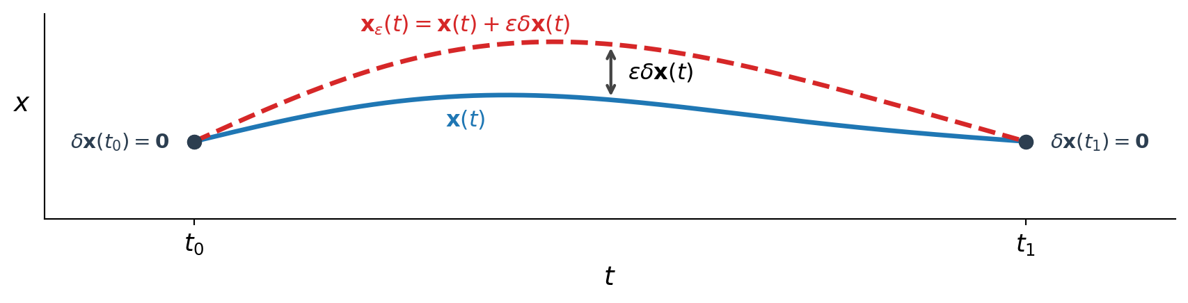
Consider a family of perturbed trajectories

\[ \mathbf x_\varepsilon(t) = \mathbf x(t) + \varepsilon\,\delta \mathbf x(t), \qquad \delta \mathbf x(t_0)=\delta \mathbf x(t_1)=\mathbf 0. \]

The first variation in direction \(\delta \mathbf x\) is defined by

\[ \delta \mathcal A[\mathbf x;\delta \mathbf x] := \lim_{\varepsilon\to 0}\frac{\mathcal A[\mathbf x_\varepsilon] - \mathcal A[\mathbf x]}{\varepsilon}\,, \]

1a. Variation of a functional? (cont.)

The variation can be written as a directional derivative in the space of trajectories:

\[ \delta \mathcal A[\mathbf x;\delta \mathbf x] := \left.\frac{\mathrm d}{\mathrm d\varepsilon}\mathcal A[\mathbf x_\varepsilon]\right|_{\varepsilon=0}. \]

\[ \begin{aligned} \delta \mathcal A[\mathbf x;\delta \mathbf x] &= \left.\frac{\mathrm d}{\mathrm d\varepsilon}\int_{t_0}^{t_1} L \left(\mathbf x_\varepsilon,\frac{\mathrm d \mathbf x_\varepsilon}{\mathrm d t},t \right)\,\mathrm dt\right|_{\varepsilon=0} \\[1mm] &=\left.\int_{t_0}^{t_1} \left(\frac{\partial L}{\partial \mathbf x}\cdot \frac{\mathrm d}{\mathrm d\varepsilon}\mathbf x_\varepsilon + \frac{\partial L}{\partial \dot{\mathbf x}}\cdot \frac{\mathrm d}{\mathrm d\varepsilon}\frac{\mathrm d \mathbf x_\varepsilon}{\mathrm d t}\right)\,\mathrm dt\right|_{\varepsilon=0} \\[1mm] &=\int_{t_0}^{t_1} \left(\frac{\partial L}{\partial \mathbf x}\cdot \delta \mathbf{x} + \frac{\partial L}{\partial \dot{\mathbf x}}\cdot \frac{\mathrm d \delta \mathbf x}{\mathrm dt}\right)\,\mathrm dt \\[1mm] &=\int_{t_0}^{t_1} \left(\frac{\partial L}{\partial \mathbf x} - \frac{\mathrm d}{\mathrm dt}\frac{\partial L}{\partial \dot{\mathbf x}}\right) \cdot \delta \mathbf{x}\,\mathrm dt + \left.\frac{\partial L}{\partial \dot{\mathbf x}}\cdot \delta \mathbf x\right|_{t_0}^{t_1} \end{aligned} \]

Hamilton’s principle states that critical trajectories satisfy

\[ \delta \mathcal A[\mathbf x;\delta \mathbf x] = 0 \quad\text{for all admissible }\delta \mathbf x. \]

1b. Why use variational principles?

• One scalar object generates the full dynamics:

\[ \mathcal A[\mathbf x] = \int_{t_0}^{t_1} L(\mathbf x,\dot{\mathbf x},t)\,\mathrm dt \]

• Constraints are handled systematically, for example with multipliers:

\[ \delta \int_{t_0}^{t_1} \big(L(\mathbf x,\dot{\mathbf x},t) + \lambda(t)\,g(\mathbf x,t)\big)\,\mathrm dt = 0 \]

• Symmetry and conservation are linked directly through invariance of the action.

\[ \textrm{symmetry of }\mathcal A\quad\Longleftrightarrow\quad\text{conserved quantity} \]

• Leads to structure-preserving discretizations, discussed in Part II.

1d. Conservation laws from variational structure

For \(L = L(t,\mathbf x,\dot{\mathbf x})\quad\,\), one obtains the identity

\[ \begin{aligned} \frac{\mathrm d}{\mathrm dt}\left(\dot{\mathbf x} \cdot \frac{\partial L}{\partial \dot{\mathbf x}} - L\right) &= \ddot{\mathbf x} \cdot \frac{\partial L}{\partial \dot{\mathbf x}} + \dot{\mathbf x} \cdot \frac{\mathrm d}{\mathrm dt} \frac{\partial L}{\partial \dot{\mathbf x}} - \dot{\mathbf x} \cdot \frac{\partial L}{\partial \mathbf x} - \ddot{\mathbf x} \cdot \frac{\partial L}{\partial \dot{\mathbf x}} - \frac{\partial L}{\partial t} \\ &= -\frac{\partial L}{\partial t} \end{aligned} \]

Therefore, if there is no explicit time dependence,

\[ \frac{\partial L}{\partial t}=0 \qquad\Longrightarrow\qquad E := \dot{\mathbf x} \cdot \frac{\partial L}{\partial \dot{\mathbf x}} - L, \quad \frac{\mathrm dE}{\mathrm dt}=0 \]

If a coordinate is cyclic, one gets momentum conservation:

\[ \frac{\partial L}{\partial \mathbf x}=0 \qquad\Longrightarrow\qquad \frac{\mathrm d}{\mathrm dt}\left(\frac{\partial L}{\partial \dot{\mathbf x}}\right)=0\,,\qquad p := \frac{\partial L}{\partial \dot{\mathbf x}}, \quad \frac{\mathrm dp}{\mathrm dt}=0 \]

1e. Example: particle in a central potential

Consider a particle of mass \(m\,\) in a central potential \(V(r)\,\,\) in polar coordinates \((r,\varphi)\,\,\,\).

\[ |\dot{\mathbf x}|^2 = \dot r^2 + r^2\dot\varphi^2 \qquad\Longrightarrow\qquad L(r,\varphi,\dot r,\dot\varphi) = \frac{m}{2}\!\left(\dot r^2 + r^2\dot\varphi^2\right) - V(r) \]

Energy conservation — \(L\) has no explicit time dependence (\(\partial L/\partial t = 0\quad\)):

\[ E = \dot r\,\frac{\partial L}{\partial \dot r} + \dot\varphi\,\frac{\partial L}{\partial \dot\varphi} - L = \frac{m}{2}\!\left(\dot r^2 + r^2\dot\varphi^2\right) + V(r), \qquad \frac{\mathrm dE}{\mathrm dt} = 0 \]

Angular-momentum conservation — \(\varphi\) is cyclic (\(\partial L/\partial \varphi = 0\quad\)):

\[ \frac{\partial L}{\partial \varphi} = 0 \qquad\Longrightarrow\qquad \ell = \frac{\partial L}{\partial \dot\varphi} = m r^2\dot\varphi, \qquad \frac{\mathrm d\ell}{\mathrm dt} = 0 \]

Two symmetries of \(\mathcal A\,\,\) yield two conserved quantities — without solving any equation of motion!

2. Variational principles for PDEs (field theories)

For a field \(u(t,\mathbf x)\,\,\,\) on spacetime \([t_0,t_1]\times\Omega\quad\), consider the action

\[ \mathcal A[u] = \int_{t_0}^{t_1}\int_\Omega \mathcal L\big(u,\partial_t u,\nabla u,t,\mathbf x\big)\,\mathrm d\mathbf x\,\mathrm dt. \]

An admissible variation is a perturbation

\[ u_\varepsilon(t,\mathbf x) = u(t,\mathbf x) + \varepsilon\,\eta(t,\mathbf x), \qquad \eta = 0 \text{ on the spacetime boundary.} \]

The first variation is defined by

\[ \delta \mathcal A[u;\eta] := \left.\frac{\mathrm d}{\mathrm d\varepsilon}\mathcal A[u_\varepsilon]\right|_{\varepsilon=0}. \]

2. Variational principles for PDEs (field theories, cont.)

Computing the derivative gives

\[ \delta \mathcal A[u;\eta] = \int_{t_0}^{t_1}\int_\Omega \left( \frac{\partial \mathcal L}{\partial u}\,\eta + \frac{\partial \mathcal L}{\partial (\partial_t u)}\,\partial_t \eta + \frac{\partial \mathcal L}{\partial (\nabla u)}\cdot\nabla \eta \right)\,\mathrm d\mathbf x\,\mathrm dt. \]

After integration by parts in time and space,

\[ \delta \mathcal A[u;\eta] = \int_{t_0}^{t_1}\int_\Omega \left( \frac{\partial \mathcal L}{\partial u} - \partial_t\frac{\partial \mathcal L}{\partial (\partial_t u)} - \nabla\cdot\frac{\partial \mathcal L}{\partial (\nabla u)} \right)\eta\,\mathrm d\mathbf x\,\mathrm dt. \]

Thus stationarity for all admissible \(\eta\,\) yields the field Euler-Lagrange equation

\[ \frac{\partial \mathcal L}{\partial u} - \partial_t\frac{\partial \mathcal L}{\partial (\partial_t u)} - \nabla\cdot\frac{\partial \mathcal L}{\partial (\nabla u)} = 0. \]

2a. Example: Poisson equation from an action

Let \(\phi(\mathbf x)\,\,\) be a scalar field on \(\Omega\,\) and consider

\[ \mathcal A[\phi] = \int_\Omega \left( \frac{|\nabla \phi|^2}{2} - \rho\,\phi\right)\,\mathrm d\mathbf x. \]

Take variations

\[ \phi_\varepsilon = \phi + \varepsilon\,\eta, \qquad \eta|_{\partial\Omega}=0. \]

Then

\[ \delta \mathcal A[\phi;\eta] = \left.\frac{\mathrm d}{\mathrm d\varepsilon}\mathcal A[\phi_\varepsilon]\right|_{\varepsilon=0} = \int_\Omega \left(\nabla\phi\cdot\nabla\eta - \rho\,\eta\right)\,\mathrm d\mathbf x. \]

2a. Example: Poisson equation from an action (cont.)

Integrating by parts and using \(\eta|_{\partial\Omega}=0\),

\[ \int_\Omega \nabla\phi\cdot\nabla\eta\,\mathrm d\mathbf x = -\int_\Omega \Delta\phi\,\eta\,\mathrm d\mathbf x. \]

Therefore

\[ \delta \mathcal A[\phi;\eta] = \int_\Omega \left(-\,\Delta\phi - \rho\right)\eta\,\mathrm d\mathbf x. \]

Stationarity for all \(\eta\) gives

\[ -\,\Delta\phi - \rho = 0 \qquad\Longleftrightarrow\qquad -\Delta\phi = \rho. \]

3. Lagrangian vs. Eulerian descriptions of fluid motion

Let \(\mathbf u(t,\mathbf x)\quad\) be the fluid velocity field at any given time \(t\) at position \(\mathbf x\).

Lagrangian description (particle-following):

Track each fluid parcel labeled by its initial position \(\mathbf x_0\).

\[ \begin{aligned} \frac{\mathrm d}{\mathrm dt}\Phi_t(\mathbf x_0) &= \mathbf u\big(t,\Phi_t(\mathbf x_0)\big), \qquad \Phi_0(\mathbf x_0)=\mathbf x_0. \\[1mm] \frac{\mathrm d^2}{\mathrm dt^2}\Phi_t(\mathbf x_0) &= \frac 1m \mathbf F\big(t,\Phi_t(\mathbf x_0)\big) \end{aligned} \]

• \(\Phi_t(\mathbf x_0)\,\,\,\) is the position at time \(t\) of the fluid parcel that started at \(\mathbf x_0\) at time \(0\).

• \(\mathbf F(t, \mathbf x)\,\,\,\) is the force acting on the fluid parcel at position \(\mathbf x\) at time \(t\).

• For each \(t \in [t_0,t_1]\quad\), the mapping \(\Phi_t:\Omega \to \Omega\quad\) is a diffeomorphism. \(\Phi_t\,\) is called the flow map and encodes the full fluid motion.

3. Lagrangian vs. Eulerian descriptions of fluid motion (cont.)

Eulerian description (field-at-fixed-point):

Observe the mass density \(\rho(t,\mathbf x)\,\,\,\) at fixed spatial location \(\mathbf x\,\). For compressible flow, this yields

\[ \begin{aligned} \partial_t\rho + \nabla\cdot(\rho\mathbf u) &= 0, \\[2mm] \partial_t\mathbf u + (\mathbf u\cdot\nabla)\mathbf u &= \frac{1}{\rho} \mathbf F(t,\mathbf x). \end{aligned} \]

• solve a system of PDEs (!) for \(\rho(t,\mathbf x)\,\,\,\) and \(\mathbf u(t,\mathbf x)\)

Bridge between both views: The Lagrangian parcel acceleration equals the Eulerian material derivative:

\[ \frac{\mathrm d}{\mathrm dt}\mathbf u\big(t,\Phi(t,\mathbf x_0)\big) = \big(\partial_t + \mathbf u\cdot\nabla\big)\mathbf u. \]

3a. Lagrangian vs. Eulerian sketches

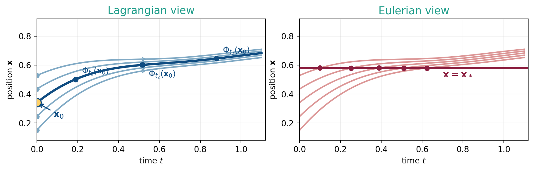
Lagrangian viewpoint

• Move with the flow (follow parcels)
• Unknown: trajectory / flow map \(\Phi_t(\mathbf x_0)\)
• Label parcels by initial position \(\mathbf x_0\)
• Question: where does this parcel go?
• Solve ODEs for \(\Phi_t(\mathbf x_0)\,\,\,\) for different \(\mathbf x_0\)

Eulerian viewpoint

• Stay at a fixed location \(\mathbf{x}_*\)
• Unknowns: fields \(\rho(t,\mathbf x),\,\mathbf u(t,\mathbf x)\)
• Label points by spatial location \(\mathbf x\)
• Question: what passes through?
• Solve PDEs for \(\rho(t,\mathbf x),\,\mathbf u(t,\mathbf x)\)

4. Euler-Poincaré reduction

Suppose we have a Lagrangian description of fluid motion in terms of the flow map \(\Phi_t(\mathbf x_0)\,\,\,\) for all \(\mathbf x_0 \in \Omega \subset \mathbb R^3:\)

\[ \begin{aligned} \frac{\mathrm d}{\mathrm dt}\Phi_t(\mathbf x_0) &= \mathbf u\big(t,\Phi_t(\mathbf x_0)\big), \qquad \Phi_0(\mathbf x_0)=\mathbf x_0. \\[1mm] \frac{\mathrm d^2}{\mathrm dt^2}\Phi_t(\mathbf x_0) &= - \frac 1m \nabla V\big(\Phi_t(\mathbf x_0)\big) \end{aligned} \]

From what we have learned so far it is easy to write down a variational principle for this Lagrangian description for a fixed initial position \(\mathbf x_0:\)

\[ \mathcal A_\textrm{Lagrange}(\Phi_t, \dot{\Phi}_t) = \int_0^T \left( m\frac{|\dot{\Phi}_t(\mathbf x_0)|^2}{2} - V\big(\Phi_t(\mathbf x_0)\big) \right) \,\mathrm dt. \]

Can we write down an equivalent variational principle for the Eulerian description?

4a. Local conservation of mass

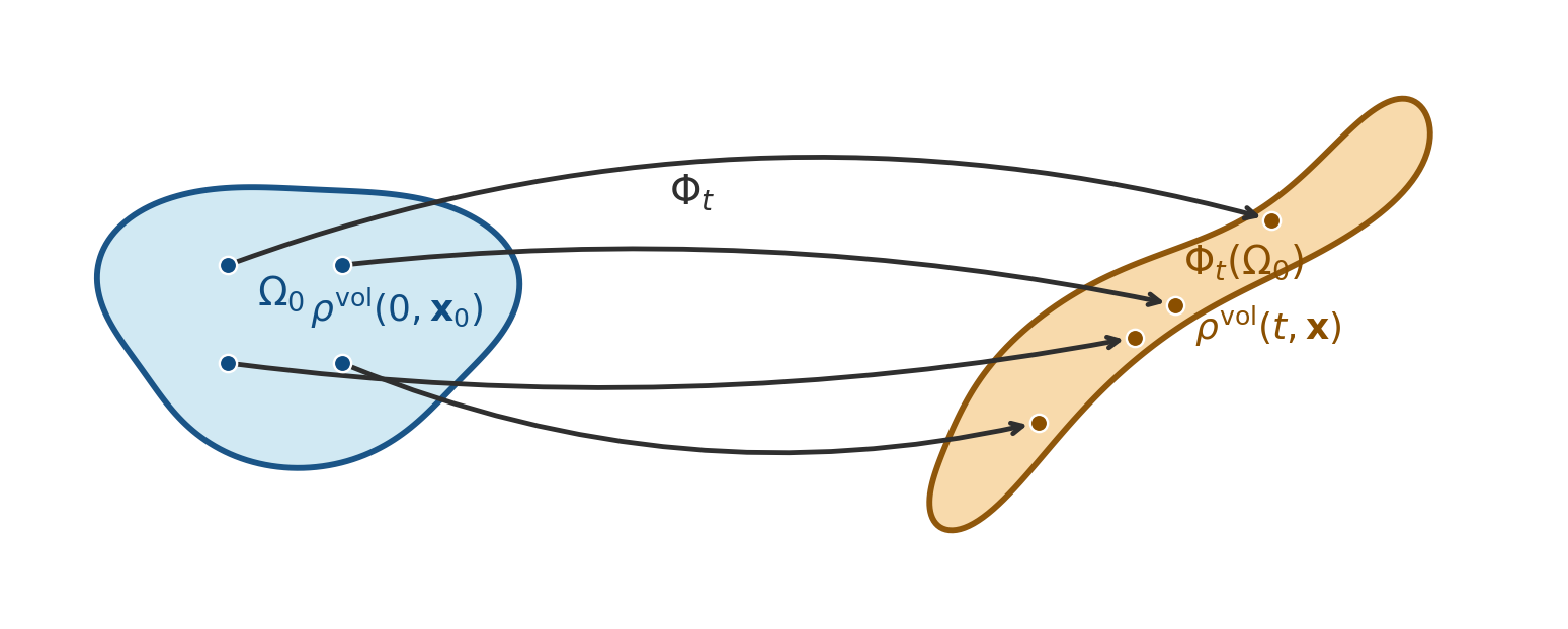
A volume form assigns to any open subset \(\Omega \subset \mathbb R^3\quad\) a real number:

\[ \rho^\textrm{vol}:\quad \Omega \subset_\textrm{open} \mathbb R^3 \mapsto \int_\Omega \rho^\textrm{vol}(\mathbf x)\,\textrm d \mathbf x \in \mathbb R. \]

A density (transported by the flow) is a time-dependent volume form that is invariant under the flow \(\Phi_t:\)

\[ \int_{\Phi_t(\Omega_0)} \rho^\textrm{vol}(t, \mathbf x)\,\textrm d \mathbf x = \int_{\Omega_0} \rho^\textrm{vol}(0, \mathbf x_0)\,\textrm d \mathbf x_0\qquad \forall \,\Omega_0. \]

4a. Local conservation of mass (cont.)

1. A density satisfies the continuity equation:

\[ \frac{\partial \rho^\textrm{vol}}{\partial t} + \nabla \cdot (\rho^\textrm{vol} \mathbf u) = 0. \]

where \(\mathbf u(t, \mathbf x):= \dot{\Phi}_t \circ \Phi_t^{-1}(\mathbf x)\qquad\,\) is the Eulerian velocity field, which follows from \(\mathbf x = \Phi_t(\mathbf x_0).\)

2. The following is constant along the flow:

\[ \frac{\mathrm d}{\mathrm dt} \Big[ \rho^\textrm{vol}(\Phi_t) \,\big| \textrm{det} D\Phi_t\big| \Big] = 0. \]

3. The variation of a density is given by

\[ \delta \rho^\textrm{vol} = -\nabla \cdot (\rho^\textrm{vol} \boldsymbol\eta). \]

for arbitrary vector field \(\boldsymbol\eta(t, \mathbf x):= \delta \Phi_t \circ \Phi_t^{-1}(\mathbf x).\)

4b. From Lagrangian to Eulerian coordinates

Assume an initial mass density \(\rho^\textrm{vol}(0, \mathbf x_0)\quad\) and consider the modified Lagrange action

\[ \mathcal A_\textrm{Lagrange}(\Phi_t, \dot{\Phi}_t) = \int_0^T \int_{\Omega_0} \left( \frac{|\dot{\Phi}_t(\mathbf x_0)|^2}{2} - \frac 1m V\big(\Phi_t(\mathbf x_0)\big) \right) \rho^\textrm{vol}(0, \mathbf x_0) \, \textrm d \mathbf x_0\,\mathrm dt. \]

Using the change of variables \(\mathbf x = \Phi_t(\mathbf x_0)\quad\), as well as the dynamics given by
\(\dot{\Phi}_t(\mathbf x_0) = \mathbf u(t, \Phi_t(\mathbf x_0))\qquad\,\,\,\), we get

\[ \mathcal A_\textrm{Euler}(\mathbf u, \ldots) = \int_0^T \int_{\Omega} \left( \frac{|\mathbf u(t, \mathbf x)|^2}{2} - \frac 1m V(\mathbf x) \right) \frac{\rho^\textrm{vol}(0, \Phi_t^{-1}(\mathbf x))}{ \big| \textrm{det} D\Phi_t(\Phi_t^{-1}(\mathbf x)) \big|} \, \textrm d \mathbf x\,\mathrm dt \]

We can now use 2. from the previous slide, namely

\[ \rho^\textrm{vol}(t, \Phi_t(\mathbf x_0)) = \frac{\rho^{\textrm{vol}}(0, \mathbf x_0)}{\big| \textrm{det} D\Phi_t(\mathbf x_0) \big|} \]

4b. From Lagrangian to Eulerian

\[ \mathcal A_\textrm{Euler}(\mathbf u, \rho^\textrm{vol}) = \int_0^T \int_{\Omega} \left( \frac{|\mathbf u(t, \mathbf x)|^2}{2} - \frac 1m V(\mathbf x) \right) \rho^\textrm{vol}(t, \mathbf x) \, \textrm d \mathbf x\,\mathrm dt \]

The unknown flow map \(\Phi_t\,\) has thus been replaced by the two unknown fields \(\mathbf u(t, \mathbf x)\,\,\,\) and \(\rho^\textrm{vol}(t, \mathbf x)\quad\). These fields have to be determined by variation of the new action.

We already know the variations of the density \(\rho^\textrm{vol}\,\,\) from 3. in the previous slide:

\[ \delta \rho^\textrm{vol} = -\nabla \cdot (\rho^\textrm{vol} \boldsymbol\eta). \]

for arbitrary vector field \(\boldsymbol\eta(t, \mathbf x):= \delta \Phi_t \circ \Phi_t^{-1}(\mathbf x).\qquad\) We can compute the variations of the velocity field from

\[ \mathbf u(t, \mathbf x) := \dot{\Phi}_t \circ \Phi_t^{-1}(\mathbf x) \]

to obtain (after some algebra)

\[ \delta \mathbf u = \partial_t \boldsymbol\eta + \mathbf u \cdot \nabla \boldsymbol\eta - \boldsymbol\eta \cdot \nabla \mathbf u. \]

4c. Computing Eulerian (constrained) variations

The Euler action:

\[ \mathcal A_\textrm{Euler}(\mathbf u, \rho^\textrm{vol}) = \int_0^T \int_{\Omega} \left( \frac{|\mathbf u(t, \mathbf x)|^2}{2} - \frac 1m V(\mathbf x) \right) \rho^\textrm{vol}(t, \mathbf x) \, \textrm d \mathbf x\,\mathrm dt \]

The constrained variations:

\[ \begin{aligned} \delta \mathbf u &= \partial_t \boldsymbol\eta + \mathbf u \cdot \nabla \boldsymbol\eta - \boldsymbol\eta \cdot \nabla \mathbf u, \\[2mm] \delta \rho^\textrm{vol} &= -\nabla \cdot (\rho^\textrm{vol} \boldsymbol\eta). \end{aligned} \]

The computation:

\[ \delta \mathcal A_\textrm{Euler} = \underbrace{\int_0^T \int_{\Omega} \mathbf u \cdot \delta \mathbf u \, \rho^\textrm{vol} \, \textrm d \mathbf x\,\mathrm dt}_{\text{①}} + \underbrace{\int_0^T \int_{\Omega} \left( \frac{|\mathbf u|^2}{2} - \frac 1m V \right) \delta \rho^\textrm{vol} \, \textrm d \mathbf x\,\mathrm dt}_{\text{②}} \]

4c. Computing Eulerian (constrained) variations (cont.)

First integral:

\[ \begin{aligned} \text{①} = \int_0^T \int_{\Omega} \mathbf u \cdot \delta \mathbf u \, \rho^\textrm{vol} \, \textrm d \mathbf x\,\mathrm dt &= \int_0^T \int_{\Omega} \mathbf u \cdot \left( \partial_t \boldsymbol\eta + \mathbf u \cdot \nabla \boldsymbol\eta - \boldsymbol\eta \cdot \nabla \mathbf u \right) \rho^\textrm{vol} \, \textrm d \mathbf x\,\mathrm dt \\[2mm] &= \int_0^T \int_{\Omega} \left[ - \frac{\partial}{\partial t}(\rho^\textrm{vol} \mathbf u) - \nabla \cdot (\rho^\textrm{vol} \mathbf u \mathbf u^\top) - \rho^\textrm{vol} \nabla \frac{|\mathbf u|^2}{2} \right] \cdot \boldsymbol \eta \, \textrm d \mathbf x\,\mathrm dt \end{aligned} \]

Second integral:

\[ \begin{aligned} \text{②} = \int_0^T \int_{\Omega} \left( \frac{|\mathbf u|^2}{2} - \frac 1m V \right) \delta \rho^\textrm{vol} \, \textrm d \mathbf x\,\mathrm dt &= - \int_0^T \int_{\Omega} \left( \frac{|\mathbf u|^2}{2} - \frac 1m V \right) \nabla \cdot (\rho^\textrm{vol} \boldsymbol\eta) \, \textrm d \mathbf x\,\mathrm dt \\[2mm] &= \int_0^T \int_{\Omega} \left[ \rho^\textrm{vol} \nabla \left( \frac{|\mathbf u|^2}{2} - \frac 1m V \right) \right] \cdot \boldsymbol\eta \, \textrm d \mathbf x\,\mathrm dt \end{aligned} \]

4c. Computing Eulerian (constrained) variations (cont.)

Hamilton’s principle \(\text{①} + \text{②} = 0\quad\) for arbitrary \(\boldsymbol\eta\,\) yields Euler’s equation for the fluid velocity field:

\[ \frac{\partial}{\partial t}(\rho^\textrm{vol} \mathbf u) + \nabla \cdot (\rho^\textrm{vol} \mathbf u \mathbf u^\top) = - \frac{\rho^\textrm{vol}}{m} \nabla V. \]

The mass conservation law is given by our assumption that \(\rho^\textrm{vol}\,\) is a density transported by the flow:

\[ \frac{\partial \rho^\textrm{vol}}{\partial t} + \nabla \cdot (\rho^\textrm{vol} \mathbf u) = 0. \]

Part II: Discretization - Particle methods for fluid Lagrangians

5. Overview

• 5a. Approximating a density by particles
• 5b. Approximating integrals by particles (Monte-Carlo)
• 5c. Constant weights
• 5d. Comparing the two approaches
• 5e. Example: Pressure-less fluids in a given potential
• 5f. Density estimation and smoothing

5a. Approximating a density by particles

A density \(\rho^\textrm{vol}\,\,\,\) satisfies

\[ \int_{\Phi_t(\Omega_0)} \rho^\textrm{vol}(t, \mathbf x)\,\textrm d \mathbf x = \int_{\Omega_0} \rho^\textrm{vol}(0, \mathbf x_0)\,\textrm d \mathbf x_0\qquad \forall \,\Omega_0. \]

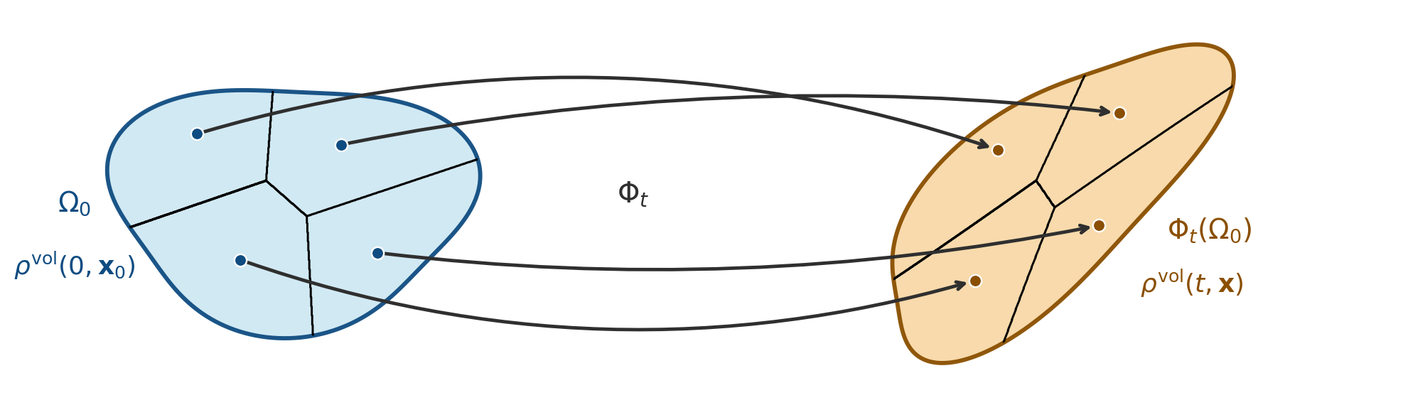
Divide the initial domain \(\Omega_0\,\) into small subregions such that \(\bigcup_i \Omega_0^i = \Omega_0:\)

5a. Approximating a density by particles (cont.)

Define the weights \(w_i \in \mathbb R\quad\) for each subregion \(\Omega_0^i\,\) by

\[ w_i := \int_{\Omega_0^i} \rho^\textrm{vol}(0, \mathbf x_0)\,\textrm d \mathbf x_0 \]

such that

\[ \sum_i w_i = \int_{\Omega_0} \rho^\textrm{vol}(0, \mathbf x_0)\,\textrm d \mathbf x_0 \]

Now let \(\mathbf x_0^i \in \Omega_0^i\quad\), then

\[ \mathbf x^i(t) = \Phi_t(\mathbf x_0^i) \quad \in \Phi_t(\Omega_0^i) \qquad \forall t \in [0, T]. \]

5a. Approximating a density by particles (cont.)

Particle approximation: We can approximate the density \(\rho^\textrm{vol}(t, \mathbf x)\quad\) at time \(t\) by a sum of weighted delta distributions centered at the particle locations \(\mathbf x^i(t):\)

\[ \rho^\textrm{vol}(t, \mathbf x) \approx \rho_N(t, \mathbf x) := \sum_{i=1}^N w_i\, \delta(\mathbf x - \mathbf x^i(t)). \]

The discrete \(\rho_N\,\) is still a density (!) since

\[ \int_{\Phi_t(\Omega_0)} \rho_N(t, \mathbf x)\,\textrm d \mathbf x = \sum_{i=1}^N w_i = \int_{\Omega_0} \rho^\textrm{vol}(0, \mathbf x_0)\,\textrm d \mathbf x_0. \]

5a. Approximating a density by particles (cont.)

The particles are advected by the flow,

\[ \mathbf x^i(t) = \Phi_t(\mathbf x_0^i),\quad \Longleftrightarrow \quad \dot{\mathbf x}^i(t) = \mathbf u(t, \mathbf x^i(t))\quad \mathbf x^i(0) = \mathbf x_0^i. \]

The weights \(w_i\,\) are constant in time, since they are defined by the initial density \(\rho^\textrm{vol}(0, \mathbf x_0)\quad\) and the partition of the initial domain \(\Omega_0\,\) into subregions \(\Omega_0^i.\)

The equation for the acceleration of the particels can be derived from a variational principle.

5b. Approximating integrals by particles (Monte-Carlo)

Suppose we aim to compute the integral

\[ I = \int_\Omega A(\mathbf x)\,\rho^\textrm{vol}(\mathbf x)\,\textrm d \mathbf x. \]

for some function (or \(0\,\)-form) \(A(\mathbf x)\,\,\). Further, suppose \(s^\textrm{vol}\,\) denotes a probability density supported on \(\Omega\,\) such that

\[ s^\textrm{vol}(\mathbf x) > 0\quad\forall\mathbf x \in \Omega,\qquad \int_\Omega s^\textrm{vol}(\mathbf x)\,\textrm d \mathbf x = 1. \]

Then we can rewrite the integral \(I\,\) as an expectation value \(\mathbb E\,\) with respect to \(s^\textrm{vol}\,:\)

\[ I = \int_\Omega A(\mathbf x)\frac{\rho^\textrm{vol}(\mathbf x)}{s^\textrm{vol}(\mathbf x)} s^\textrm{vol}(\mathbf x)\,\textrm d \mathbf x = \mathbb E\left[ A\frac{\rho^\textrm{vol}}{s^\textrm{vol}} \right]_{s^\textrm{vol}} \]

5b. Monte-Carlo (cont.)

Monte Carlo approximation. Draw \(N\,\) independent samples \(\mathbf x_i \sim s^\textrm{vol}\quad\) and approximate

\[ I \approx I_N := \frac{1}{N}\sum_{i=1}^N A(\mathbf x_i)\frac{\rho^\textrm{vol}(\mathbf x_i)}{s^\textrm{vol}(\mathbf x_i)} = \frac 1N \sum_{i=1}^N w_i A(\mathbf x_i). \]

with weights

\[ w_i = \frac{\rho^\textrm{vol}(\mathbf x_i)}{s^\textrm{vol}(\mathbf x_i)}. \]

The sample mean \(I_N\,\) can be viewed as a random variable itself, when viewing the samples \(\mathbf x_i\,\) as random variables distributed according to \(s^\textrm{vol}\,\). It is an unbiased estimator of the true mean value (which is our integral):

\[ \mathbb E[I_N] = \mathbb E\left[ \frac 1N \sum_{i=1}^N w_i A(\mathbf x_i) \right] = \frac 1N \sum_{i=1}^N \mathbb E\left[w_i A(\mathbf x_i) \right] = \frac{NI}{N} = I. \]

5b. Approximating integrals by particles (Monte-Carlo, cont.)

The variance of \(I_N\,\) is given by

\[ \mathbb V[I_N] = \mathbb E\!\left[(I_N - \mathbb E[I_N])^2\right] = \mathbb E\!\left[(I_N - I)^2\right] \]

and is a good measure for the error. Using Bienaymé’s identity for independent random variables \(X_i,\)

\[ \mathbb V\!\left[\sum_{i=1}^N X_i\right] = \sum_{i=1}^N \mathbb V[X_i], \]

5b. Approximating integrals by particles (Monte-Carlo, cont.)

We can estimate the rate of convergence of the Monte Carlo approximation:

\[ \begin{aligned} \mathbb V[I_N] &= \mathbb V\left[ \frac 1N \sum_{i=1}^N w_i A(\mathbf x_i) \right] \\[2mm] &= \frac{1}{N^2} \mathbb V\left[ \sum_{i=1}^N w_i A(\mathbf x_i) \right] \\[2mm] &= \frac{1}{N^2} \left[ \sum_{i=1}^N \mathbb V[w_i A(\mathbf x_i)] \right] = \frac{N \sigma^2}{N^2} = \frac{\sigma^2}{N}. \end{aligned} \]

where \(\sigma\,\) is the standard deviation of the random variable \(w_i A(\mathbf x_i)\quad\).

5b. Approximating integrals by particles (Monte-Carlo, cont.)

Hence the root-mean-square error decays as

\[ \boxed{\varepsilon_N := \sqrt{\mathbb E\!\left[(I_N - I)^2\right]} = \frac{\sigma}{\sqrt{N}}} \]

independent of the spatial dimension \(d\) — this is the key advantage of Monte Carlo over quadrature rules, which converge as \(N^{-k/d}\,\,\,\) for smooth \(k\,\)-th order rules.

5c. Constant weights

In the Monte-Carlo approximation, the weights \(w_i\,\) are given by

\[ w_i(t) = \frac{\rho^\textrm{vol}(t, \mathbf x_i(t))}{s^\textrm{vol}(t, \mathbf x_i(t))}, \]

where \(\mathbf x_i(t) = \Phi_t(\mathbf x_0^i)\qquad\) are the particle locations at time \(t\,\). We can make the following observations:

• \(\rho^\textrm{vol}\,\,\) is a density and thus

\[ \rho^\textrm{vol}(t, \mathbf x_i(t)) = \frac{\rho^\textrm{vol}(0, \mathbf x_0^i)}{\big| \textrm{det} D\Phi_t(\mathbf x_0^i) \big|}. \]

5c. Constant weights (cont.)

• \(s^\textrm{vol}\,\,\) is an arbitrary probability density supported on \(\Omega\,\). We can choose it to be transported by the flow as well, i.e. 

\[s^\textrm{vol}(t, \mathbf x_i) = \frac{s^\textrm{vol}(0, \mathbf x_0^i)}{\big| \textrm{det} D\Phi_t(\mathbf x^i_0) \big|}. \]

This implies constancy of the weights:

\[ w_i(t) = \frac{\rho^\textrm{vol}(t, \mathbf x_i(t))}{s^\textrm{vol}(t, \mathbf x_i(t))} = \frac{\rho^\textrm{vol}(0, \mathbf x_0^i)}{s^\textrm{vol}(0, \mathbf x_0^i)} = w_i(0) = const. \]

5c. Constant weights (cont.)

Hence, in the Monte-Carlo approach, one draws the initial samples \(\mathbf x_0^i\,\) from a probability density \(s^\textrm{vol}(0, \mathbf x_0)\quad\). The information about the initial density \(\rho^\textrm{vol}(0, \mathbf x_0)\quad\) is encoded in the constant weights \(w_i\,\). The particles are then transported by the flow,

\[ \mathbf x^i(t) = \Phi_t(\mathbf x_0^i),\quad \Longleftrightarrow \quad \dot{\mathbf x}^i(t) = \mathbf u(t, \mathbf x^i(t))\quad \mathbf x^i(0) = \mathbf x_0^i, \]

and the weights remain constant.

The equation for the acceleration of the particels can be derived from a variational principle.

5d. Comparing the two approaches

The particle approximation of the density \(\rho^\textrm{vol}(t, \mathbf x)\quad\) is given by

\[ \rho_N(t, \mathbf x) = \sum_{i=1}^N w_i\, \delta(\mathbf x - \mathbf x^i(t)). \]

where the markers are transported by the flow,

\[ \mathbf x^i(t) = \Phi_t(\mathbf x_0^i) \]

and the weights remain constant.

The same discrete ansatz is obtained from two different constructions of the initial markers and weights.

5d. Comparing the two approaches

	Density approach	Monte-Carlo approach
Drawing the markers	Partition \(\Omega_0\) into grid cells \(\Omega_0^i\) and place one marker at the cell center \(\mathbf x_0^i \in \Omega_0^i\quad\). The initial markers are therefore distributed regularly.	Draw the initial markers randomly and independently, \(\mathbf x_0^i \sim s^\textrm{vol}(0, \mathbf x_0)\quad\,\,\). The initial markers therefore follow the sampling density \(s^\textrm{vol}\).
Weights	\(w_i := \int_{\Omega_0^i} \rho^\textrm{vol}(0, \mathbf x_0)\,\textrm d\mathbf x_0\).	\(w_i := \dfrac 1N \dfrac{\rho^\textrm{vol}(0, \mathbf x_0^i)}{s^\textrm{vol}(0, \mathbf x_0^i)}\)
Comments	Needs numerical quadrature over the initial cells.	Lots of noise, but provable convergence of integrals \(\sim 1/\sqrt N\,\,\,\).

5e. Example: Pressure-less fluids in a given potential

We can now discretize the action in Eulerian coordinates,

\[ \mathcal A_\textrm{Euler}(\mathbf u, \rho^\textrm{vol}) = \int_0^T \int_{\Omega} \left( \frac{|\mathbf u(t, \mathbf x)|^2}{2} - \frac 1m V(\mathbf x) \right) \rho^\textrm{vol}(t, \mathbf x) \, \textrm d \mathbf x\,\mathrm dt \]

by substituting the particle approximation

\[ \rho^\textrm{vol}(t, \mathbf x) \approx \rho_N(t, \mathbf x) = \sum_{i=1}^N w_i\, \delta(\mathbf x - \mathbf x^i(t)) \]

to obtain …

5e. Example: Pressure-less fluids in a given potential (cont.)

\[ \begin{aligned} \mathcal A(\mathbf u, \mathbf x^1, \ldots, \mathbf x^N) &= \int_0^T \int_{\Omega} \left( \frac{|\mathbf u(t, \mathbf x)|^2}{2} - \frac 1m V(\mathbf x) \right) \rho_N(t, \mathbf x) \, \textrm d \mathbf x\,\mathrm dt \\[2mm] &= \sum_{i=1}^N w_i \int_0^T \left( \frac{|\mathbf u(t, \mathbf x^i(t))|^2}{2} - \frac 1m V(\mathbf x^i(t)) \right) \, \mathrm dt \\[2mm] &= \sum_{i=1}^N w_i \int_0^T \left( \frac{|\dot{\mathbf x}^i(t)|^2}{2} - \frac 1m V(\mathbf x^i(t)) \right) \, \mathrm dt \end{aligned} \]

where we used the fact that the particles are advected by the flow, i.e. \(\dot{\mathbf x}^i(t) = \mathbf u(t, \mathbf x^i(t)).\)

5e. Example (cont.)

The action has been reduced to a sum of \(N\,\) independent single-particle actions. The dynamics of the system is thus given by \(N\,\) independent copies of the single-particle dynamics in the potential \(V(\mathbf x)\,\,\,\) i.e. \(N\,\) independent solutions of Newton’s equation

\[ \ddot{\mathbf x}^i = -\frac{1}{m}\nabla V(\mathbf x^i). \]

By contrast, an Eulerian (grid-based) discretization of the same problem would require the discretization of

\[ \begin{aligned} \frac{\partial \rho^\textrm{vol}}{\partial t} + \nabla \cdot (\rho^\textrm{vol} \mathbf u) &= 0 \\[2mm] \frac{\partial \mathbf u}{\partial t} + \mathbf u \cdot \nabla \mathbf u &= - \frac{1}{m} \nabla V \end{aligned} \]

which features nonlinear terms and requires the solution of a coupled system of equations at each time step.

5f. Density estimation and smoothing

At each time \(t\,\) we have

\[ \rho_N(t, \mathbf x) = \sum_{i=1}^N w_i\, \delta(\mathbf x - \mathbf x^i(t)). \]

But the true solution of the PDE is smooth.

• How to evaluate the density?
• How to visualize it?
• How to compute derivatives of the density?

We can obtain a smoother approximation by convolution of \(\rho_N\,\) with a smoothing kernel \(W_h\,\) (e.g. a Gaussian kernel with bandwidth \(h\,\)):

\[ \rho_{h,N}(t, \mathbf x) := (W_h * \rho_N)(t, \mathbf x) = \int_\Omega W_h(\mathbf x - \mathbf y) \rho_N(t, \mathbf y)\,\textrm d \mathbf y = \sum_{i=1}^N w_i\, W_h(\mathbf x - \mathbf x^i(t)). \]

5f. Density estimation (cont.)

At a chosen evaluation point \(\mathbf x^*\,\,\), the sum only includes contributions from particles within the \(h\,\)-neighborhood of \(\mathbf x^*,\)

\[ \rho_{h,N}(t, \mathbf x^*) = \sum_{i: \|\mathbf x^* - \mathbf x^i(t)\| < h} w_i\, W_h(\mathbf x^* - \mathbf x^i(t)). \]

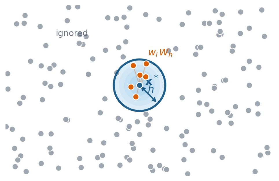
Algorithmically, we need an efficient way to query the neighboring particles for each evaluation point \(\mathbf x^*.\)

5f. Density estimation (cont.)

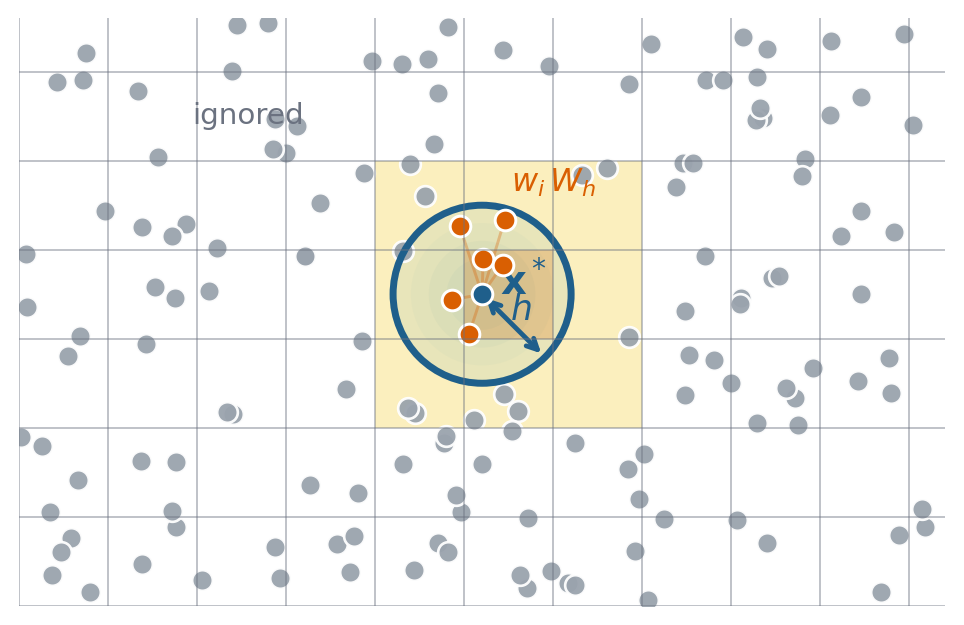
• Solution: assign particles to boxes, require box-size \(\geq h\,\,\,\), then:

  1. find box of \(\mathbf x^*\)
  2. query particles in the same box and the neighboring boxes only
  3. compute the sum over the particles in these boxes and ignore the rest

5f. Density estimation and smoothing (cont.)

The question of convergence is important:

• \(\rho_{h,N} \to \rho^\textrm{vol}\quad\,\) as \(N \to \infty\quad\) and \(h\,\) fixed ?
• \(\rho_{h,N} \to \rho^\textrm{vol}\quad\,\) as \(h \to 0\quad\) and \(Nh^3\,\,\) fixed ?

These are non-trivial questions we will answer empirically (via simulation).

Other quantities, like the velocity, can also be evaluated in a similar way, e.g.

\[ \mathbf u_{h,N}(t, \mathbf x) = \sum_i w_i\frac{\mathbf v_i(t)}{\rho_{h,N}(\mathbf x_i(t))}\,W_h(\mathbf x - \mathbf x^i(t)), \]

with \(\mathbf v_i = \mathbf u(t, \mathbf x^i(t)) = \dot{\mathbf x}^i(t)\).

Practical Part I: Marker drawing and density evaluation

Overview

We demonstrate SPH kernel density evaluation in 1D using Struphy.

Goal: recover the density \(\rho(\eta_1) = 1.5 + \cos(2\pi\eta_1)\qquad\,\,\) on \(\eta_1 \in [0,1]\quad\) from \(N\,\) markers.

Steps:

1. Define domain, background density, and perturbation
2. Create a ParticlesSPH object and draw markers
3. Initialize weights \(w_i\) from the background density
4. Evaluate the SPH density estimate \(\rho_{h,N}(\eta_1) = \sum_i w_i\,W_h(\eta_1 - \eta_1^i)\)
5. Compare with the exact solution

The corresponding test is test_sph_evaluation_1d in struphy/src/struphy/pic/tests/test_sph.py.

Target density

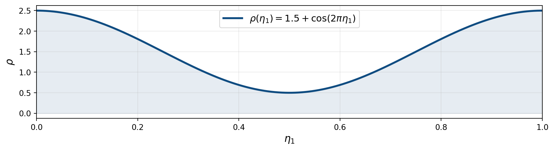
\[ \rho(\eta_1) = \underbrace{1.5}_{\text{background}} + \underbrace{\cos(2\pi\eta_1)}_{\text{perturbation}}, \qquad \eta_1 \in [0,1] \]

Step 1: Domain, background, and particles

import numpy as np

# from the Strpuhy API
from struphy import (
    BoundaryParameters, LoadingParameters, SortingParameters, domains, perturbations, equils
)

# not part of the API (loaded for this test only)
from struphy.pic.particles import ParticlesSPH

# 1D domain in logical coordinates eta1 in [0, 1]
domain = domains.Cuboid(l1=1.0, r1=2.0, l2=10.0, r2=20.0, l3=100.0, r3=200.0)

# background n=1.5 plus perturbation: rho = 1.5 + cos(2*pi*eta1)
background = equils.ConstantVelocity(n=1.5, density_profile="constant")
background.domain = domain
pert = {"n": perturbations.ModesCos(ls=(1,), amps=(1.0,))}

# tesselation: 4 markers per box placed on a regular grid
loading_params  = LoadingParameters(ppb=4, seed=1607, loading="tesselation")
boundary_params = BoundaryParameters(bc_sph=("periodic", "periodic", "periodic"))
sorting_params  = SortingParameters(boxes_per_dim=(24, 1, 1))

Step 2: Draw markers and initialize weights

particles = ParticlesSPH(
    comm_world=None,          # no MPI for this example
    loading_params=loading_params,
    boundary_params=boundary_params,
    sorting_params=sorting_params,
    bufsize=1.0,
    domain=domain,
    background=background,
    perturbations=pert,
    n_as_volume_form=True,
)

particles.draw_markers(sort=False)  # place markers at initial positions
particles.initialize_weights()      # compute w_i from background density

• draw_markers places one marker per cell center (tesselation) or draws random samples
• initialize_weights sets \(w_i = \int_{\Omega_0^i} \rho^\text{vol}(0, \mathbf x_0)\,\mathrm d\mathbf x_0\)

Step 3: Evaluate the SPH density

# evaluation grid
eta1 = np.linspace(0, 1.0, 100)
ee1, ee2, ee3 = np.meshgrid(eta1, np.array([0.0]), np.array([0.0]), indexing="ij")

# bandwidth = box size h = 1/24
h1, h2, h3 = 1.0 / 24, 1.0, 1.0

rho_sph = particles.eval_density(
    ee1, ee2, ee3,
    h1=h1, h2=h2, h3=h3,
    kernel_type="gaussian_1d",
    derivative=0,
)

rho_exact = 1.5 + np.cos(2 * np.pi * eta1)
err = np.max(np.abs(np.array(rho_sph).squeeze() - rho_exact)) / np.max(np.abs(rho_exact))
print(f"Max relative error: {err:.4f}")

Max relative error: 0.0008

Result: exact vs. SPH

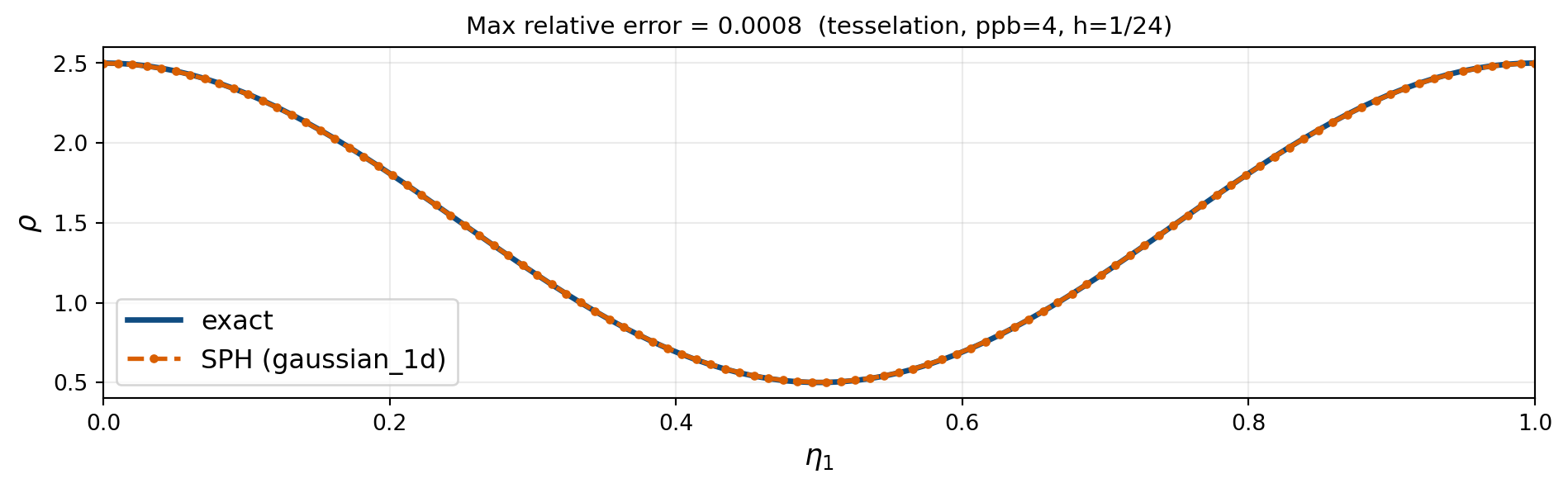
\[ \rho_{h,N}(\eta_1) = \sum_{i=1}^N w_i\, W_h(\eta_1 - \eta_1^i) \approx 1.5 + \cos(2\pi\eta_1) \]

SPH smoothing kernels

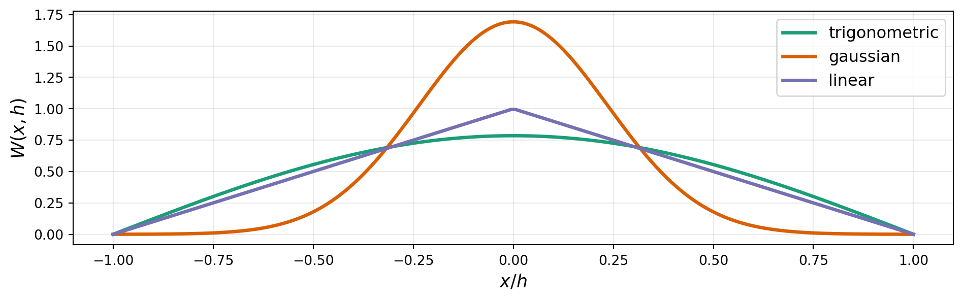
\[ \rho_{h,N}(\mathbf{x}) = \sum_i w_i\, W_h(\mathbf{x} - \mathbf{x}^i), \qquad W_h(\mathbf{x}) = \frac{1}{h}\,W\!\left(\frac{|\mathbf{x}|}{h}\right) \]

Comparing SPH kernels

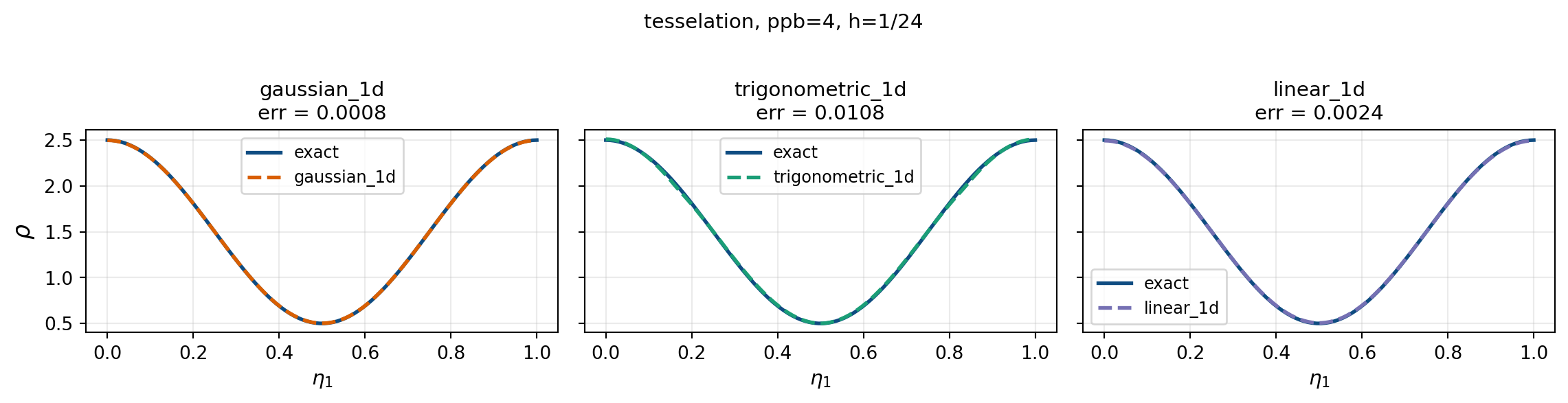
All three kernels recover the density well.

Practical Part II: 2D Density Evaluation

Overview

We extend the SPH density evaluation to 2D using Struphy.

Goal: recover \(\rho(\eta_1,\eta_2) = 1.5 + \cos(2\pi\eta_1)\cos(2\pi\eta_2)\qquad\qquad\) on \((\eta_1,\eta_2)\in[0,1]^2\quad\,\,\) from \(N\,\) markers.

Steps:

1. Define domain, background density, and 2D perturbation
2. Create a ParticlesSPH object and draw markers on a \(12\times12\quad\) grid
3. Initialize weights from the background density
4. Evaluate the 2D SPH density estimate with gaussian_2d
5. Compare with the exact solution

The corresponding test is test_sph_evaluation_2d in struphy/src/struphy/pic/tests/test_sph.py.

Target density

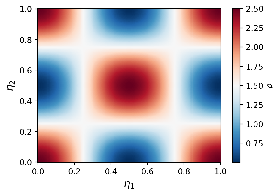
\[ \rho(\eta_1,\eta_2) = \underbrace{1.5}_{\text{background}} + \underbrace{\cos(2\pi\eta_1)\cos(2\pi\eta_2)}_{\text{perturbation}}, \qquad (\eta_1,\eta_2)\in[0,1]^2 \]

Step 1: Domain, background, and particles

# 2D domain; logical coordinates (eta1, eta2) in [0,1]^2
dom2d = domains.Cuboid(l1=1.0, r1=2.0, l2=0.0, r2=2.0, l3=100.0, r3=200.0)

# background n=1.5, perturbation: rho = 1.5 + cos(2pi*eta1)*cos(2pi*eta2)
bg2d = equils.ConstantVelocity(n=1.5, density_profile="constant")
bg2d.domain = dom2d
pert2d = {"n": perturbations.ModesCosCos(ls=(1,), ms=(1,), amps=(1.0,))}

# tesselation: 16 markers per box on a 12x12 grid
loading2d  = LoadingParameters(ppb=16, loading="tesselation")
boundary2d = BoundaryParameters(bc_sph=("periodic", "periodic", "periodic"))
sorting2d  = SortingParameters(boxes_per_dim=(12, 12, 1))

Step 2: Draw markers and initialize weights

particles2d = ParticlesSPH(
    comm_world=None,
    loading_params=loading2d,
    boundary_params=boundary2d,
    sorting_params=sorting2d,
    bufsize=1.0,
    domain=dom2d,
    background=bg2d,
    perturbations=pert2d,
    n_as_volume_form=True,
)

particles2d.draw_markers(sort=False)
particles2d.initialize_weights()

• Markers placed on a \(12\times12\quad\) tesselation grid (\(N = 12^2 \times 16 = 2304\qquad\,\) markers)
• Kernel width \(h_1 = h_2 = \tfrac{1}{12}\quad\,\) matches the box size

Step 3: Evaluate the SPH density

# evaluation grid
eta1_2d = np.linspace(0, 1.0, 50)
eta2_2d = np.linspace(0, 1.0, 50)
ee1_2d, ee2_2d, ee3_2d = np.meshgrid(eta1_2d, eta2_2d, np.array([0.0]), indexing="ij")

h2d = 1.0 / 12  # bandwidth = box size

rho_sph_2d = particles2d.eval_density(
    ee1_2d, ee2_2d, ee3_2d,
    h1=h2d, h2=h2d, h3=1.0,
    kernel_type="gaussian_2d",
    derivative=0,
)

rho_exact_2d = 1.5 + np.cos(2 * np.pi * ee1_2d) * np.cos(2 * np.pi * ee2_2d)
err_2d = np.max(np.abs(np.array(rho_sph_2d).squeeze() - rho_exact_2d.squeeze())) / np.max(np.abs(rho_exact_2d))
print(f"Max relative error: {err_2d:.4f}")

Max relative error: 0.0061

Result: exact vs. SPH

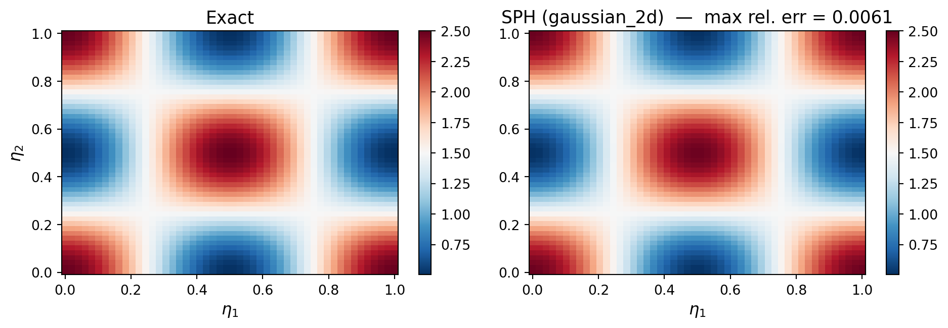
\[ \rho_{h,N}(\eta_1,\eta_2) = \sum_i w_i\, W_h(\eta_1 - \eta_1^i,\,\eta_2 - \eta_2^i) \approx 1.5 + \cos(2\pi\eta_1)\cos(2\pi\eta_2) \]

Convergence: role of \(h\) and \(N\)

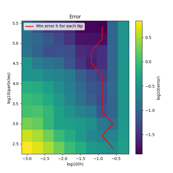
Two competing sources of error:

• Kernel width bias (large \(h\), right): kernel too wide — over-smoothing of sharp features
• Sampling variance (small \(h\), left): too few markers inside the kernel support

Optimal kernel width (red curve): trades off the two effects; as \(N\uparrow\,\) the optimal \(h\) shrinks — more markers allow a finer kernel.

Convergence: along the red curve the minimum error decreases with \(N\). Together \(h\to 0\,\,\,\), \(N\to\infty\,\,\,\,\) with \(N h^d \to\infty\) ensures \(\rho_{h,N}\to\rho\qquad\).

Pressure and Viscosity

Viscous Euler with SPH: Lagrangian discretization

Lagrangian action for the viscous Euler equations:

\[ \mathcal{A}_{\mathrm{Euler}}(\mathbf{u},\rho^{\mathrm{vol}}) = \int_0^T\!\int_{\Omega} \!\left(\frac{|\mathbf{u}(t,\mathbf{x})|^2}{2} -\frac{V(\mathbf{x})}{m} -\mathcal{U}(\rho)\right) \rho^{\mathrm{vol}}(t,\mathbf{x})\,\mathrm{d}\mathbf{x}\,\mathrm{d}t \]

Substitute the particle approximation \(\rho^{\mathrm{vol}}\approx\rho_N = \sum_{i=1}^N w_i\,\delta(\mathbf{x}-\mathbf{x}^i(t))\qquad\quad\,\,\) and use \(\mathbf{u}(t,\mathbf{x}^i(t))=\dot{\mathbf{x}}^i(t)=:\mathbf{v}_i(t)\qquad\,\,\,\,\):

\[ \mathcal{A}_N = \int_0^T\sum_{i=1}^N w_i \!\left(\frac{|\mathbf{v}_i(t)|^2}{2} -\frac{V(\mathbf{x}^i(t))}{m} -\mathcal{U}\!\left(\rho\!\left(t,\mathbf{x}^i(t)\right)\right)\right)\mathrm{d}t \]

• The action becomes a finite-dimensional integral over particle trajectories
• The term \(\mathcal{U}(\rho(t,\mathbf{x}^i))\,\,\,\,\,\) cannot be evaluated with \(\rho_N\,\,\,\) (distributional) \(\Rightarrow\,\,\,\) replace \(\rho\,\,\) by a kernel-smoothed density \(\rho_{h,N}\,\,\,\) (next slide)

Viscous Euler with SPH: Particle equations

Euler–Lagrange equations of \(\mathcal{A}_N\,\,\) (with \(\rho_{h,N}\,\,\) replacing \(\rho\,\,\)) yield the SPH particle system:

\[ \begin{aligned} \dot{\mathbf{x}}^i &= \mathbf{v}_i\,, \\[3mm] \dot{\mathbf{v}}_i &= -\frac{\nabla V(\mathbf{x}^i)}{m} \;-\; \sum_{j=1}^N w_j \!\left(\frac{\partial\mathcal{U}}{\partial\rho}(\rho_i)+\frac{\partial\mathcal{U}}{\partial\rho}(\rho_j)\right) \nabla W_h(\mathbf{x}^i-\mathbf{x}^j)\,, \end{aligned} \]

where \(\rho_i := \rho_{h,N}(t,\mathbf{x}^i) = \sum_j w_j\,W_h(\mathbf{x}^i-\mathbf{x}^j)\qquad\,\,\,\).

• External force: \(-\nabla V/m\,\,\,\,\) (gravity, external pressure gradient, …)
• Pressure force: \(-\sum_j w_j\!\left(\tfrac{\partial\mathcal{U}}{\partial\rho}(\rho_i)+\tfrac{\partial\mathcal{U}}{\partial\rho}(\rho_j)\right)\nabla W_h\qquad\,\,\,\,\,\) — the standard SPH pressure force, here derived from a variational principle
• Pair-wise anti-symmetric form ensures energy conservation and exact linear and angular momentum conservation

Internal energy choices

The thermodynamic pressure is defined by

\[ p(\rho) = \rho^2\,\frac{\partial\mathcal{U}}{\partial\rho}(\rho) \]

Isothermal: \(\mathcal{U}(\rho) = \kappa\,\ln\rho\quad\,\,\), \(\;\kappa\,\,\,\) constant \(\;\Rightarrow\;p(\rho) = \kappa\rho\)

\[ \dot{\mathbf{v}}_i = -\frac{\nabla V(\mathbf{x}^i)}{m} - \kappa\sum_{j=1}^N w_j \!\left(\frac{1}{\rho_i}+\frac{1}{\rho_j}\right) \nabla W_h(\mathbf{x}^i-\mathbf{x}^j) \]

Polytropic: \(\mathcal{U}(\rho) = \dfrac{\kappa\,\rho^{\gamma-1}}{\gamma-1}\quad\,\,\,\), \(\;\kappa\,\,\,\) polytropic constant, \(\;\gamma = C_p/C_v\quad\) adiabatic index \(\;\Rightarrow\;p(\rho) = \kappa\rho^\gamma\)

\[ \dot{\mathbf{v}}_i = -\frac{\nabla V(\mathbf{x}^i)}{m} - \kappa\sum_{j=1}^N w_j \!\left(\rho_i^{\gamma-2}+\rho_j^{\gamma-2}\right) \nabla W_h(\mathbf{x}^i-\mathbf{x}^j) \]

SPH viscous stress

The SPH velocity gradient at particle \(\boldsymbol\eta_i\) is obtained by differentiating the kernel interpolant:

\[ \nabla\mathbf{v}^{N,h}(\boldsymbol\eta_i) = \sum_l \frac{w_l}{\rho_{h,N}(\boldsymbol\eta_l)}\;\nabla W_h(\boldsymbol\eta_i - \boldsymbol\eta_l)\otimes\mathbf{v}_l \]

where \((\mathbf{a}\otimes\mathbf{b})_{jk}=a_j b_k\qquad\) is the outer product, so that \((\nabla\mathbf{v})_{jk}=\partial_j v_k\qquad\).

The deviatoric strain rate is the traceless symmetric part of \(\nabla\mathbf{v}^{N,h}\,\), scaled by dynamic viscosity \(\mu\):

\[ \boldsymbol\sigma(\boldsymbol\eta_i) =\mu\!\left[ \nabla\mathbf{v}^{N,h}(\boldsymbol\eta_i) +\bigl(\nabla\mathbf{v}^{N,h}(\boldsymbol\eta_i)\bigr)^{\!\top} -\tfrac{2}{3}\bigl(\nabla\cdot\mathbf{v}^{N,h}(\boldsymbol\eta_i)\bigr)\,\mathbf{I} \right] \]

• Symmetric: \(\boldsymbol\sigma=\boldsymbol\sigma^{\top}\)
• Traceless: \(\mathrm{tr}(\boldsymbol\sigma)=0\quad\), the isotropic divergence term cancels the trace of \(\nabla\mathbf{v}+(\nabla\mathbf{v})^\top\,\,\,\)

SPH viscous force

The SPH density at particle \(\boldsymbol\eta_i\) is

\[ \rho^{N,h}(\boldsymbol\eta_i) = \sum_l w_l\,W_h(\boldsymbol\eta_i - \boldsymbol\eta_l)\,. \]

Using the stored stress tensors, the SPH viscous force at particle \(\boldsymbol\eta_i\) reads

\[ \bigl(-\nabla\cdot\boldsymbol\Pi_{\mathrm{vis}}\bigr)^{N,h}(\boldsymbol\eta_i) = \sum_l \frac{w_l}{\rho^{N,h}(\boldsymbol\eta_l)}\;\boldsymbol\sigma(\boldsymbol\eta_l)\,\nabla W_h(\boldsymbol\eta_i-\boldsymbol\eta_l) \]

where \(\boldsymbol\sigma(\boldsymbol\eta_l)\,\nabla W_h\quad\) is the matrix–vector product of the \(3\times3\,\,\) stress tensor at \(\boldsymbol\eta_l\) with the kernel gradient.

• The 6 coefficients (symmetric) \(-w_i\,\boldsymbol\sigma(\boldsymbol\eta_i)/\rho^{N,h}(\boldsymbol\eta_i)\qquad\) are evaluated once per particle \(i\) per time step and stored in the markers array.
• Viscous particle push: \(\dot{\mathbf v}^i = \bigl(-\nabla\cdot\boldsymbol\Pi_{\mathrm{vis}}\bigr)^{N,h}(\boldsymbol\eta_i)\)

Tutorial Simulations

Hagen–Poiseuille flow (Monte Carlo loading)

• Pressure-driven viscous flow through a 2D channel
• Exact continuum solution: parabolic velocity profile \(u_x \propto R^2 - r^2\)
• SPH particles self-organize into the Poiseuille profile; no-slip boundary enforced via ghost particles
• Entropy production rate consistent with viscous dissipation (\(\kappa > 0\,\,\))
• Markers drawn by Monte Carlo sampling from the initial density

Hagen–Poiseuille flow (Tesselation loading)

• Same pressure-driven channel flow, markers placed on a regular tesselation grid
• More uniform initial marker distribution reduces density-estimate noise
• “Grid instability”, small perturbations grow into a “zig-zag” pattern

Dam break

• Free-surface gravity flow: water column collapses at \(t=0\)
• SPH handles the moving free surface naturally — no mesh, no interface tracking
• Wave propagation, bed wetting, and impact/splashing captured
• Strong test for mass conservation and positivity of density

SPH tutorial notebooks

Available in the struphy-hub/struphy repository on GitHub (tutorials/ folder):

• tutorial_beltrami_sph.ipynb
• tutorial_gas_expansion_sph.ipynb
• tutorial_viscous_euler_sph.ipynb
• tutorial_velocity_diffusion_sph.ipynb
• tutorial_hagen_poiseuille_sph.ipynb
• tutorial_dam_break_sph.ipynb